A Comparison of Seriation Methods

Author

Michael Hahsler

Introduction

This document compares the seriation methods available in package seriation using the popular Iris data set and randomize the order of the objects.

library("seriation")

data("iris")
x <- as.matrix(iris[sample(nrow(iris)), -5])
d <- dist(x)

Distance seriation

We first register more seriation methods. Some of these methods require the installation of more packages.

register_DendSer()
register_optics()
register_smacof()

The following methods will be used (a few slow methods are skipped).

methods <- sort(list_seriation_methods("dist"))

# skip slow methods
methods <- setdiff(methods, c("BBURCG", "BBWRCG", "Enumerate", "GSA"))
methods

 [1] "ARSA"           "DendSer"        "DendSer_ARc"    "DendSer_BAR"   
 [5] "DendSer_LPL"    "DendSer_PL"     "GW"             "GW_average"    
 [9] "GW_complete"    "GW_single"      "GW_ward"        "HC"            
[13] "HC_average"     "HC_complete"    "HC_single"      "HC_ward"       
[17] "Identity"       "isomap"         "isoMDS"         "MDS"           
[21] "MDS_angle"      "MDS_smacof"     "metaMDS"        "monoMDS"       
[25] "OLO"            "OLO_average"    "OLO_complete"   "OLO_single"    
[29] "OLO_ward"       "optics"         "QAP_2SUM"       "QAP_BAR"       
[33] "QAP_Inertia"    "QAP_LS"         "R2E"            "Random"        
[37] "Reverse"        "Sammon_mapping" "SGD"            "Spectral"      
[41] "Spectral_norm"  "SPIN_NH"        "SPIN_STS"       "TSP"           
[45] "VAT"

Details about the method can be found in the manual page for seriate().

We use a loop to run the function seriate() with each method and calculate criterion measures which indicate how good the order is.

orders <- list()
criterion <- list()
for (m in methods) {
  cat(m)
  tm <- system.time(orders[[m]] <- seriate(d, method = m))
  criterion[[m]] <- data.frame(time = tm[1]+tm[2], rbind(criterion(d, orders[[m]]))) 
  cat(" took", tm[1]+tm[2], "sec.\n")
}

ARSA took 2.08 sec.
DendSer took 3.799 sec.
DendSer_ARc took 2.741 sec.
DendSer_BAR took 2.504 sec.
DendSer_LPL took 2.036 sec.
DendSer_PL took 1.612 sec.
GW took 0.204 sec.
GW_average took 0.205 sec.
GW_complete took 0.235 sec.
GW_single took 0.219 sec.
GW_ward took 0.215 sec.
HC took 0.229 sec.
HC_average took 0.236 sec.
HC_complete took 0.22 sec.
HC_single took 0.204 sec.
HC_ward took 0.206 sec.
Identity took 0.2 sec.
isomap

Registered S3 method overwritten by 'vegan':
  method         from 
  reorder.hclust gclus

Warning in e$value: partial match of 'value' to 'values'

 took 0.378 sec.
isoMDS took 0.375 sec.
MDS took 0.235 sec.
MDS_angle took 0.243 sec.
MDS_smacof took 2.949 sec.
metaMDS took 2.008 sec.
monoMDS took 0.224 sec.
OLO took 0.197 sec.
OLO_average took 0.202 sec.
OLO_complete took 0.203 sec.
OLO_single took 0.2 sec.
OLO_ward took 0.203 sec.
optics took 0.211 sec.
QAP_2SUM took 0.243 sec.
QAP_BAR took 0.23 sec.
QAP_Inertia took 0.223 sec.
QAP_LS took 0.247 sec.
R2E took 0.284 sec.
Random took 0.293 sec.
Reverse took 0.22 sec.
Sammon_mapping took 0.571 sec.
SGD took 61.493 sec.
Spectral took 0.249 sec.
Spectral_norm took 0.561 sec.
SPIN_NH took 22.834 sec.
SPIN_STS took 40.876 sec.
TSP took 0.222 sec.
VAT took 0.219 sec.

criterion <- do.call(rbind, criterion)

We align the seriation orders. The reason is that an order 1, 2, 3 and 3, 2, 1 are equivalent and just an artifact of the algorithm. Aligning will reverse some orders so they are better aligned. Then we sort the orders from best to worst according to a popular seriation criterion measure called Gradient_weighted.

orders <- ser_align(orders)
best_to_worse <- order(criterion[["Gradient_weighted"]], decreasing = TRUE)

orders <- orders[best_to_worse]
criterion <- criterion[best_to_worse, ]

Comparison between methods

We can compare the seriation methods by how similar the orders are that they produce (measured using Spearman). The following code calculates distances between orders and then performs hierarchical clustering.

dst <- ser_dist(orders) 
hc <- permute(hclust(dst), order = "OLO", dist = dst)
plot(hc)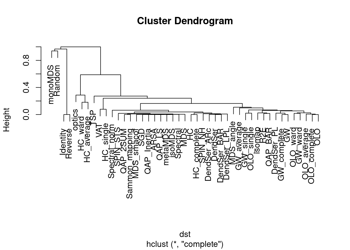

The reordered dendrogram clearly shows a group of methods based on hierarchical clustering focused on path length and another group that tries to optimize the other seriation measures.

Here is a table to compare the seriation methods on different criterion measures. Use the interactive table to sort the methods given different measures. Note that some are maximized and some should be minimized. Details about the measures can be found in the manual page for criterion().

library(DT)
datatable(round(criterion, 2), extensions = "FixedColumns",
    options = list(paging = TRUE, searching = TRUE, info = FALSE,
      sort = TRUE, scrollX = TRUE, fixedColumns = list(leftColumns = 1))) %>%
    formatRound(columns = colnames(criterion) , mark = "", digits=1)

Visualize the results

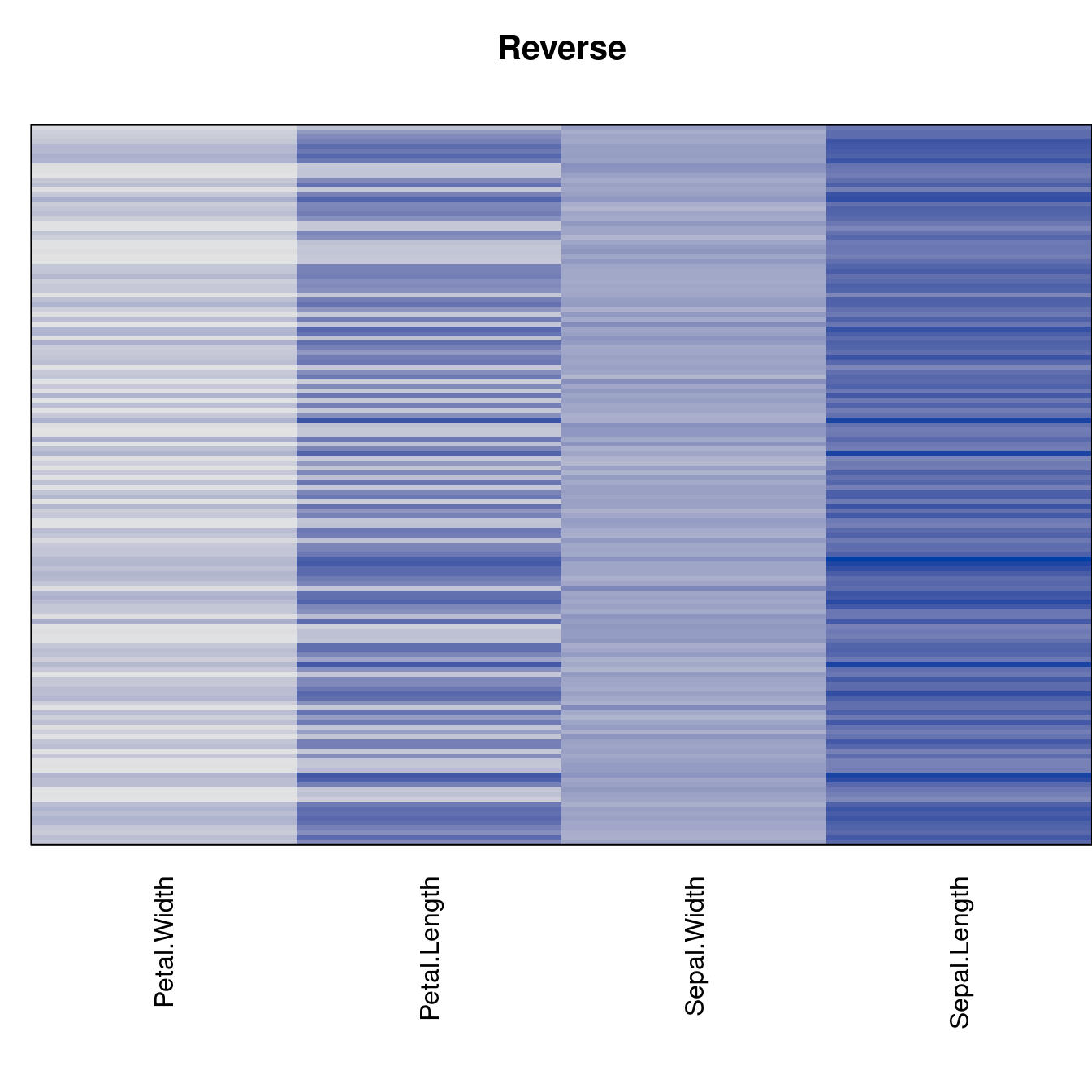
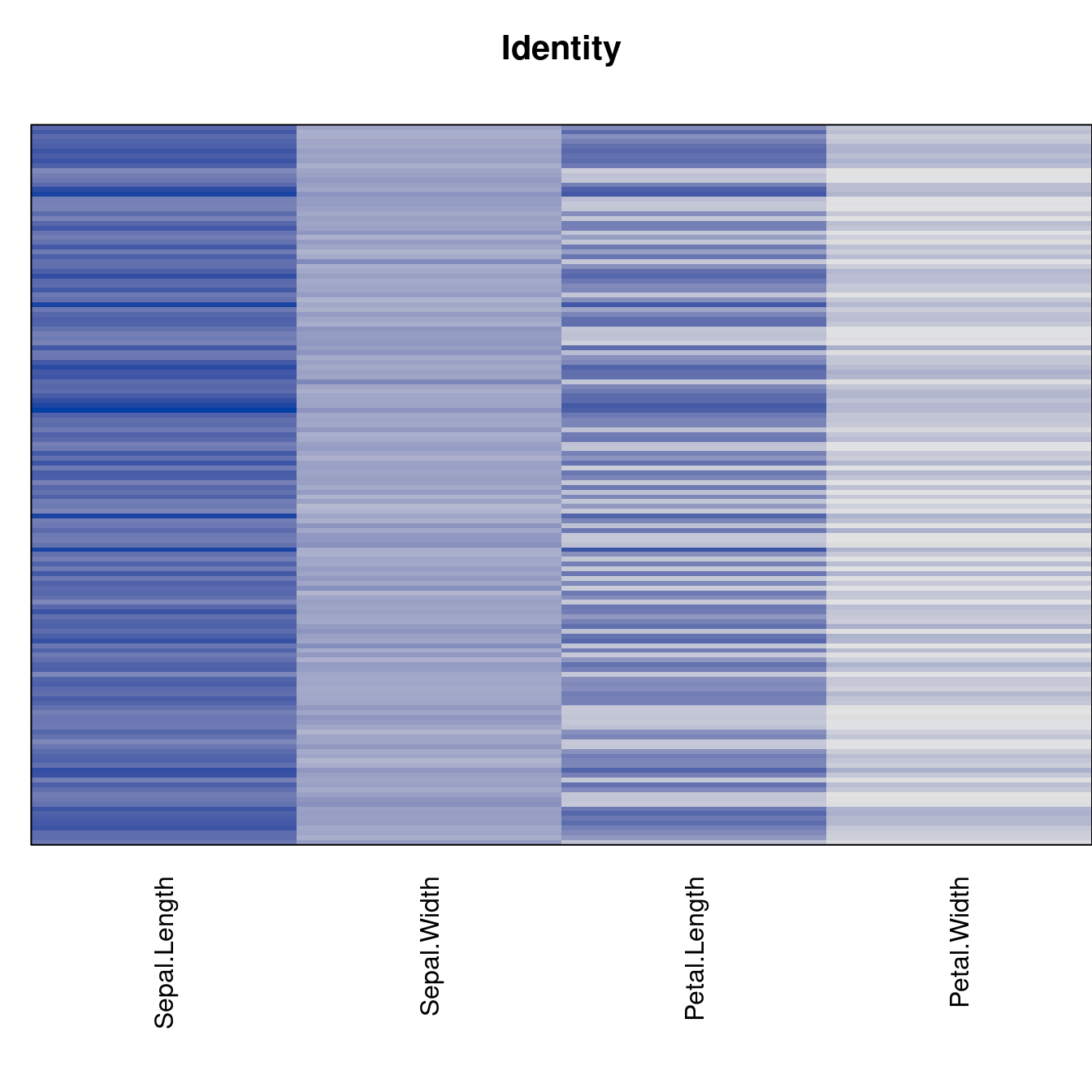
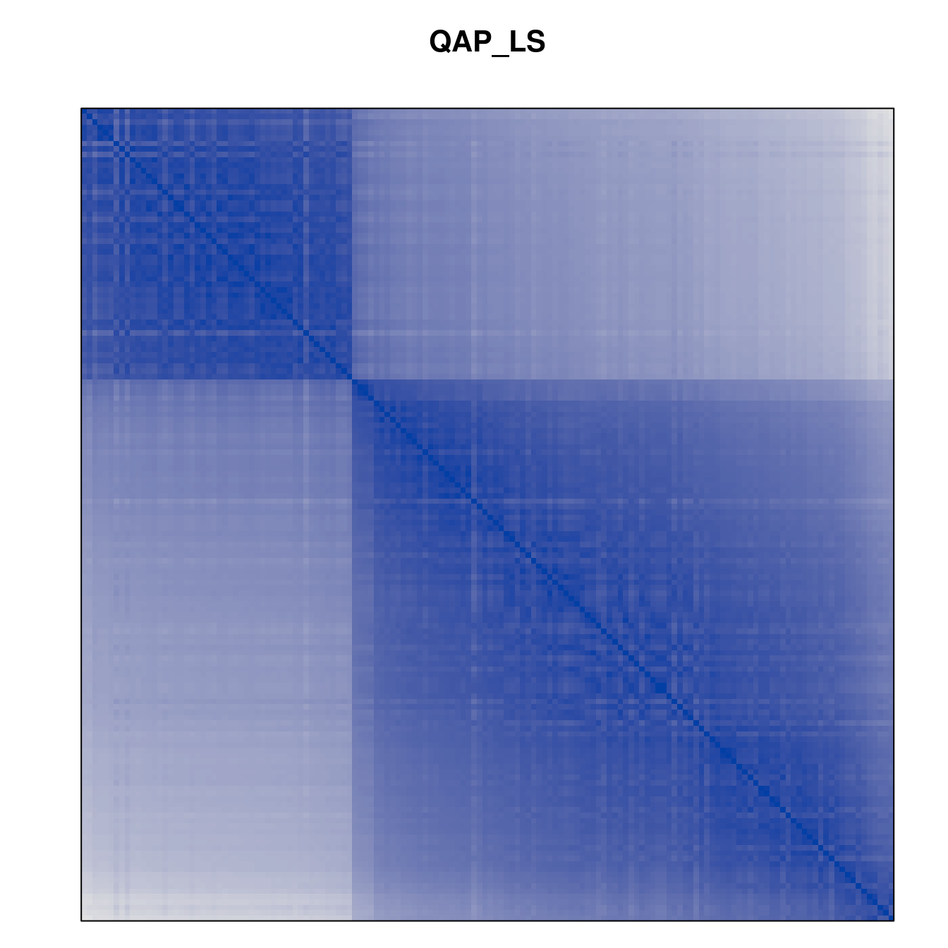
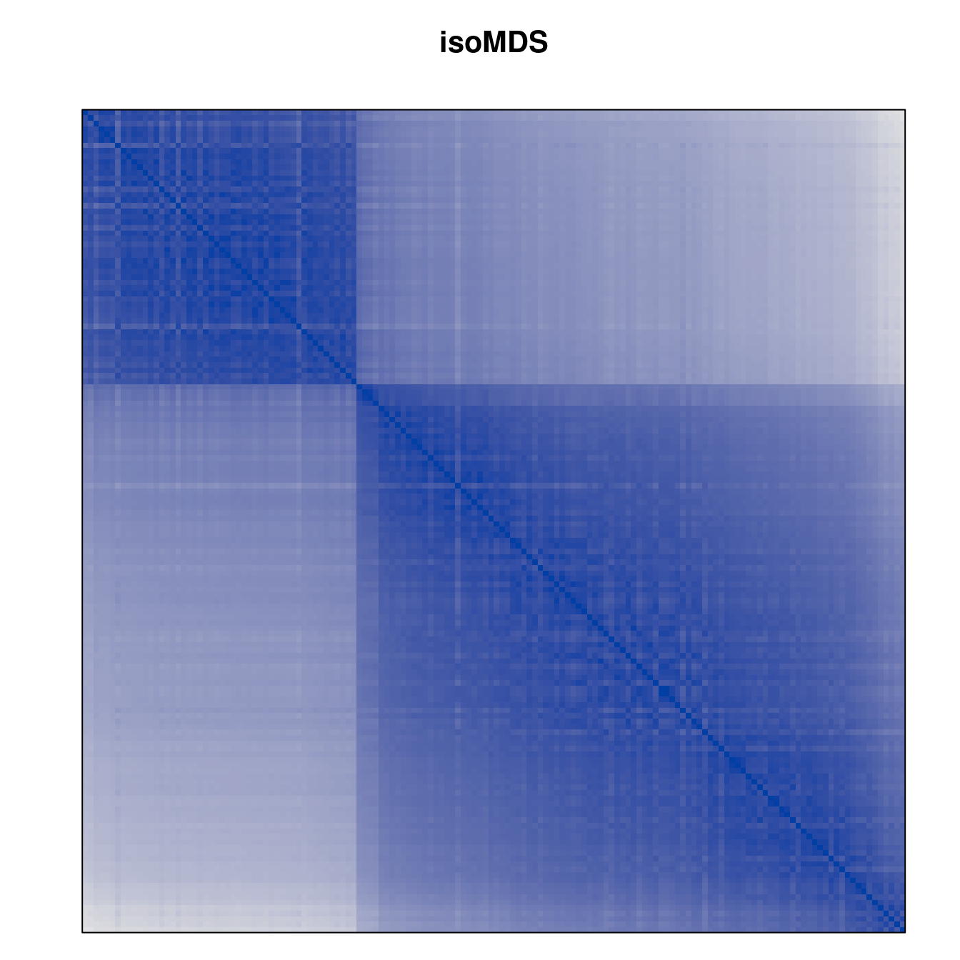
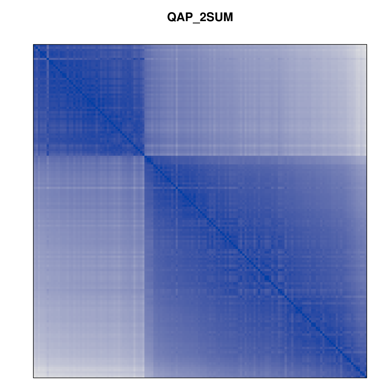
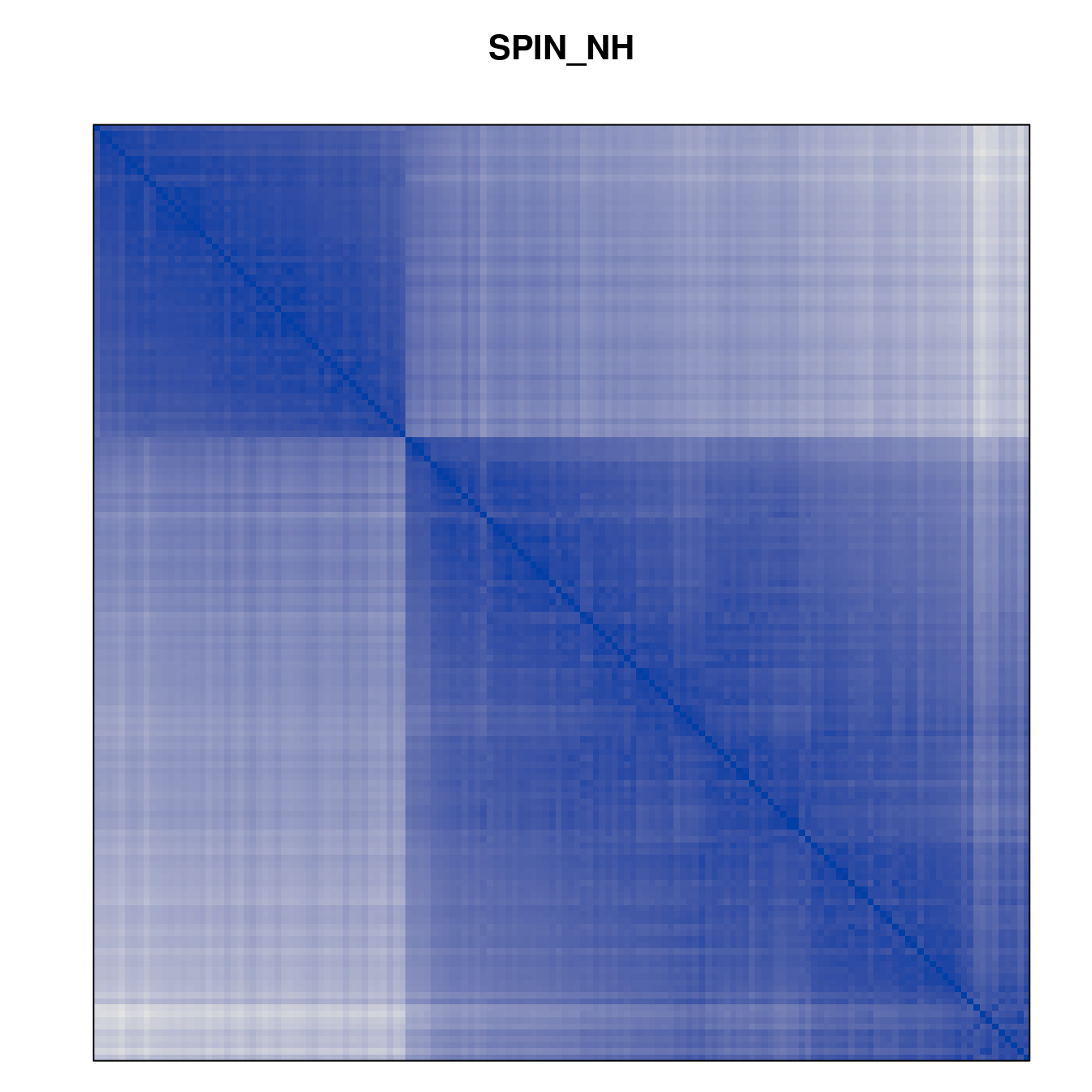
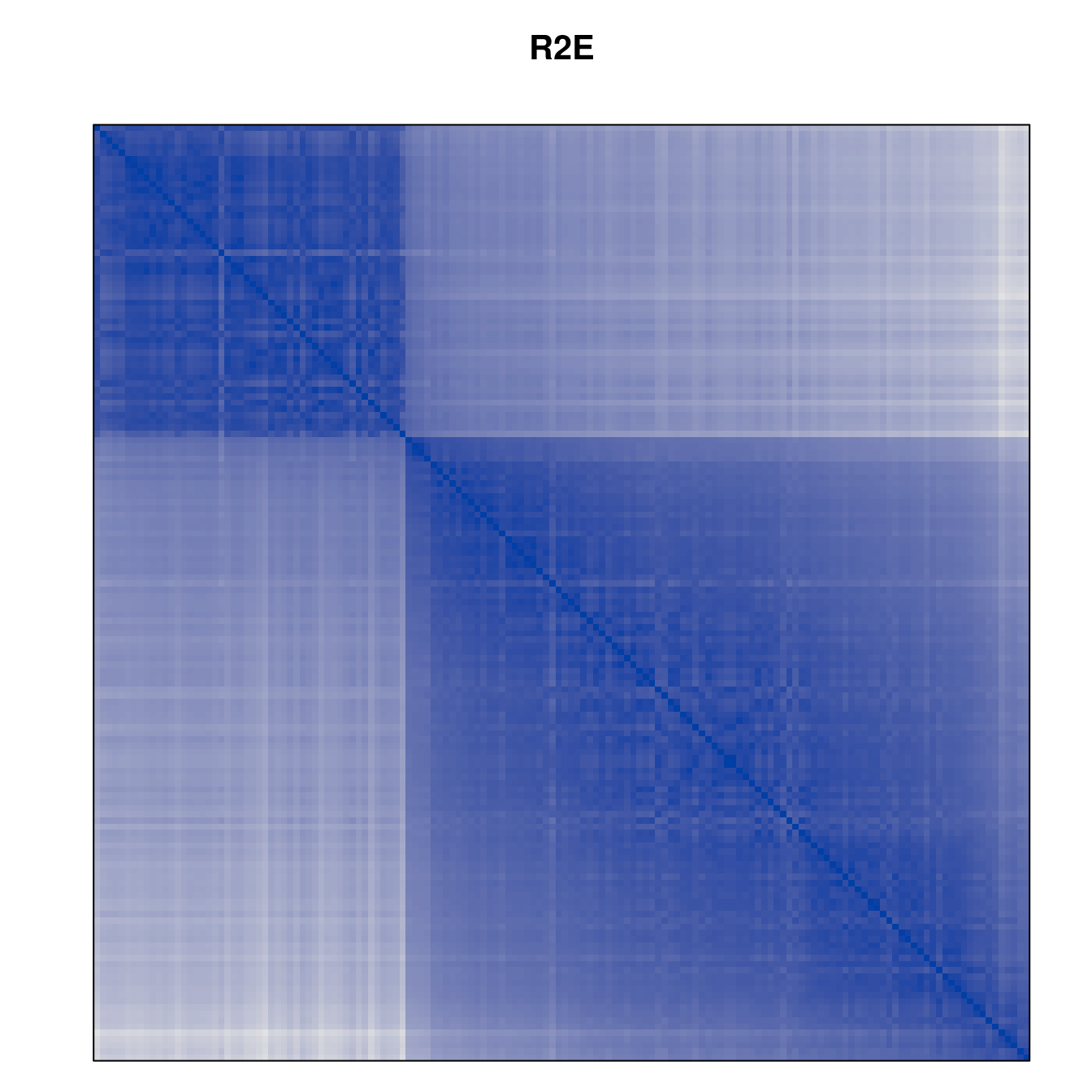
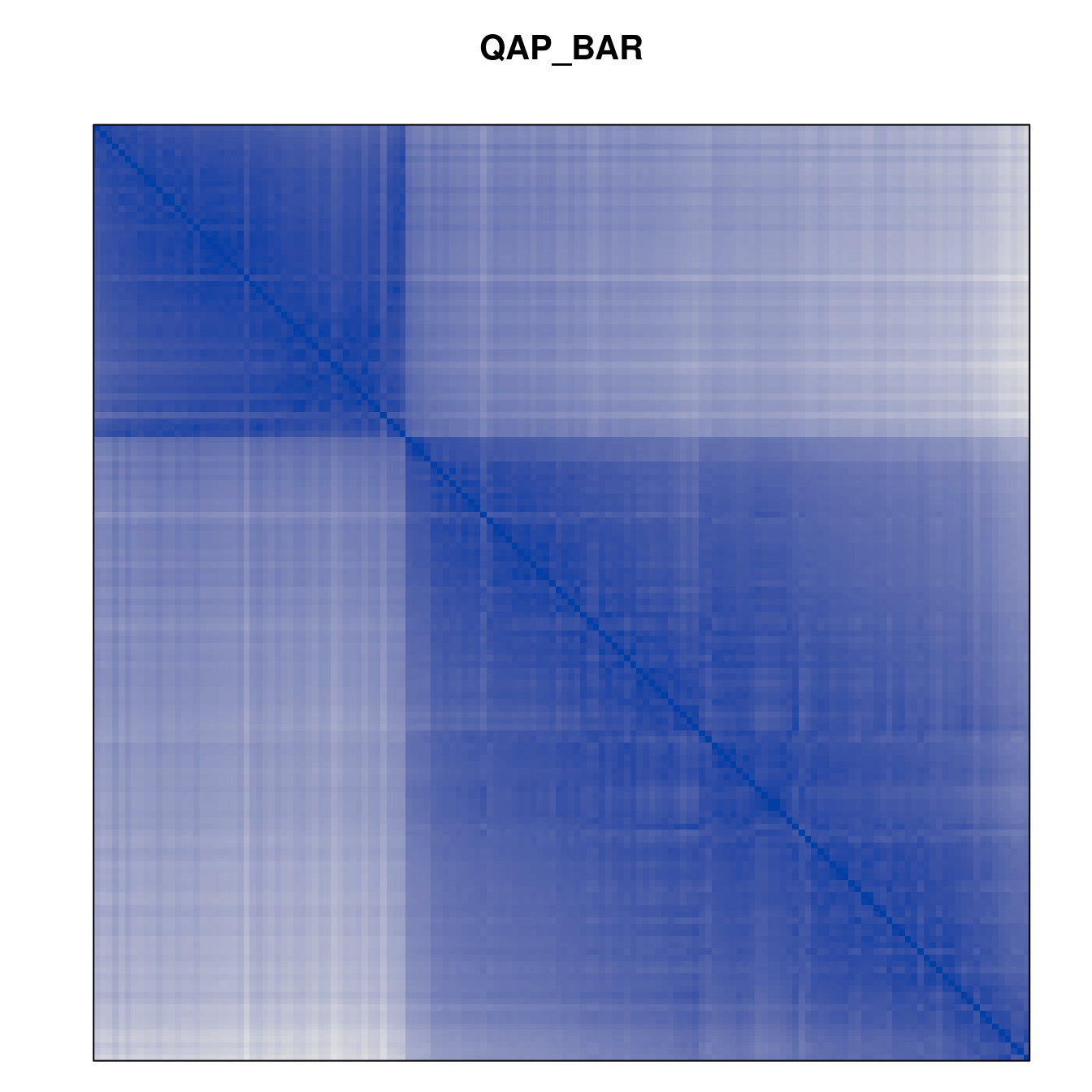
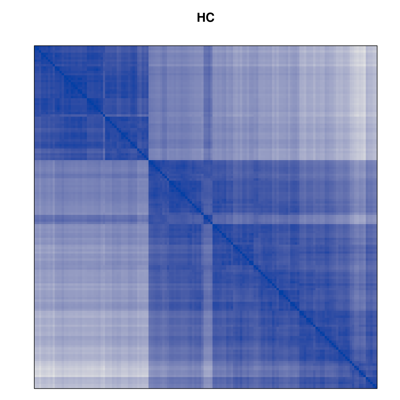
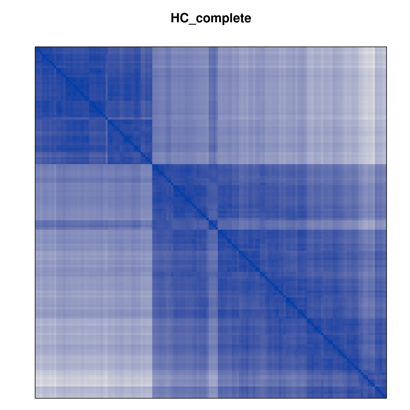
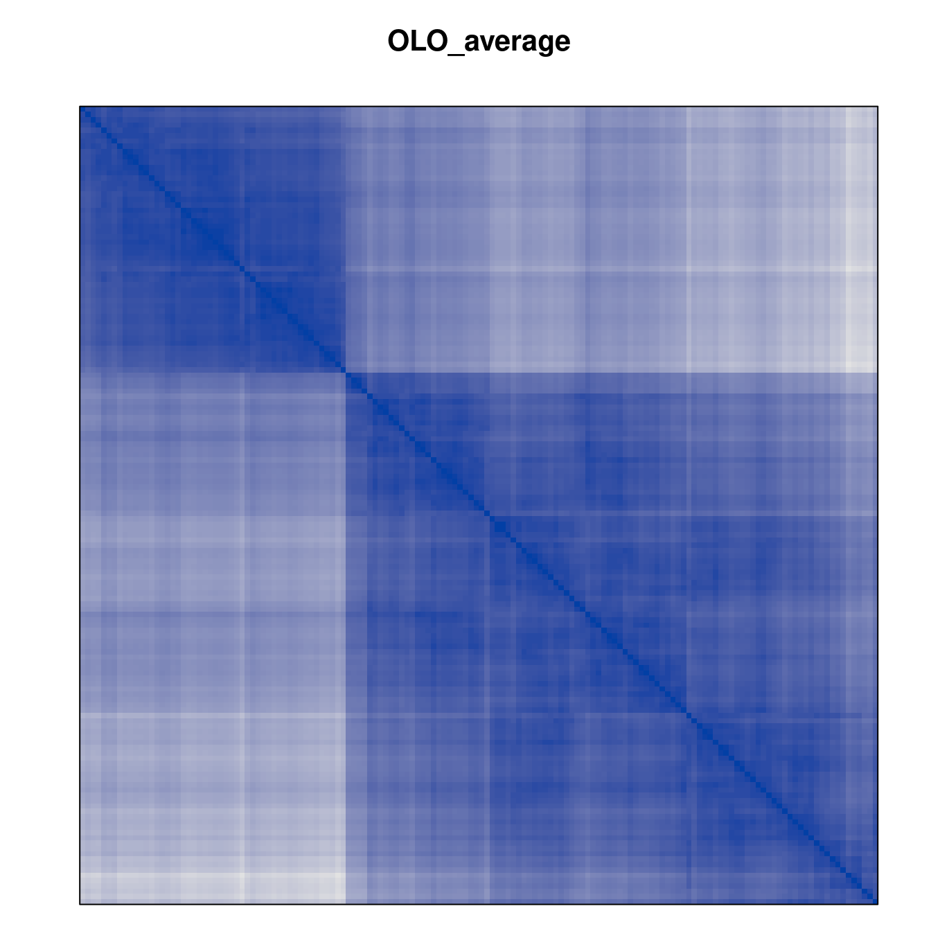
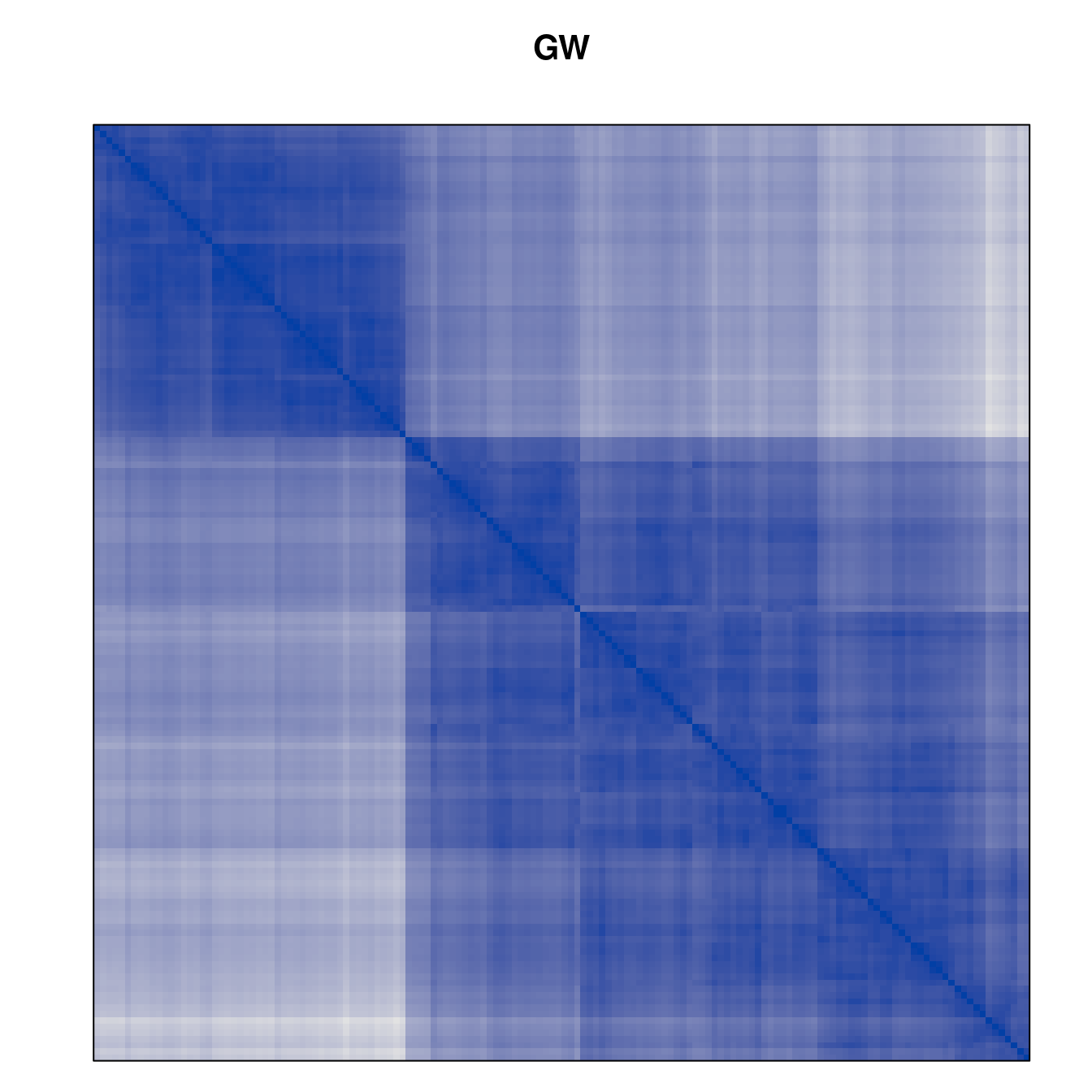
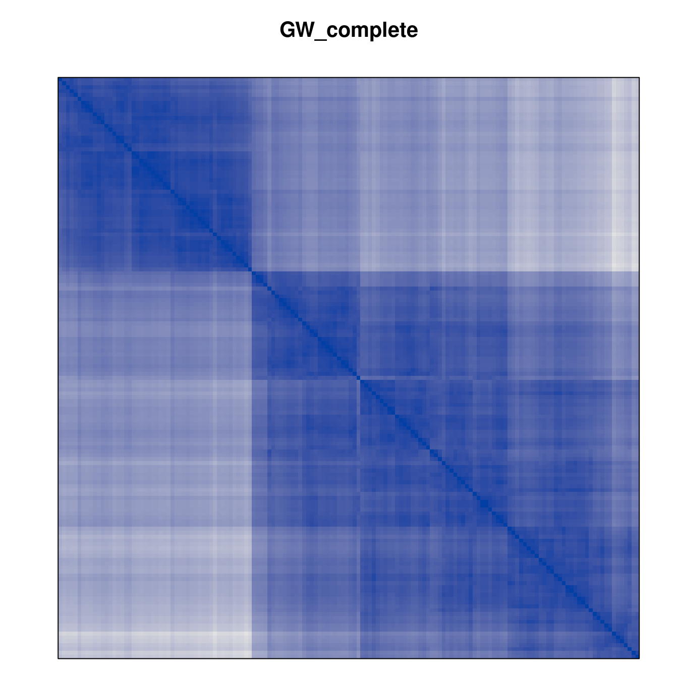
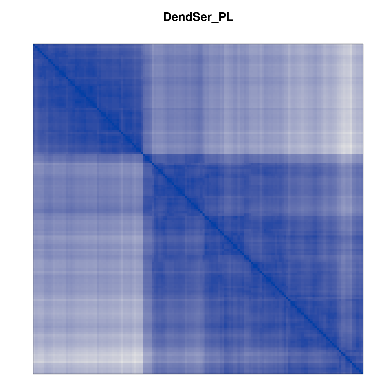
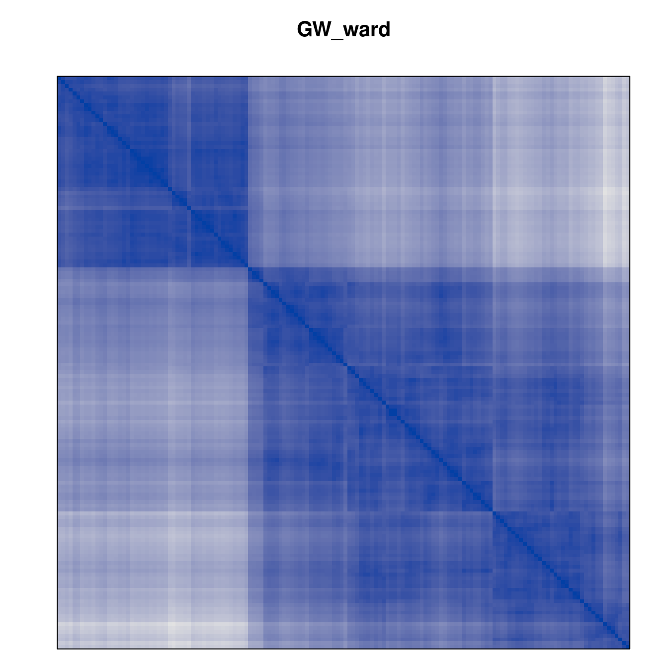
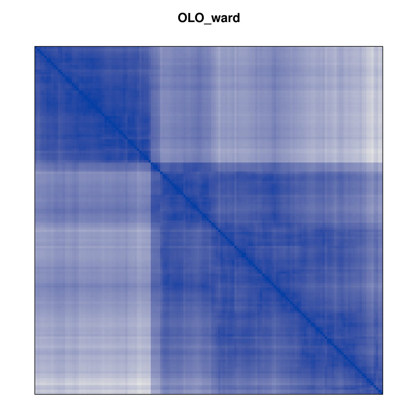
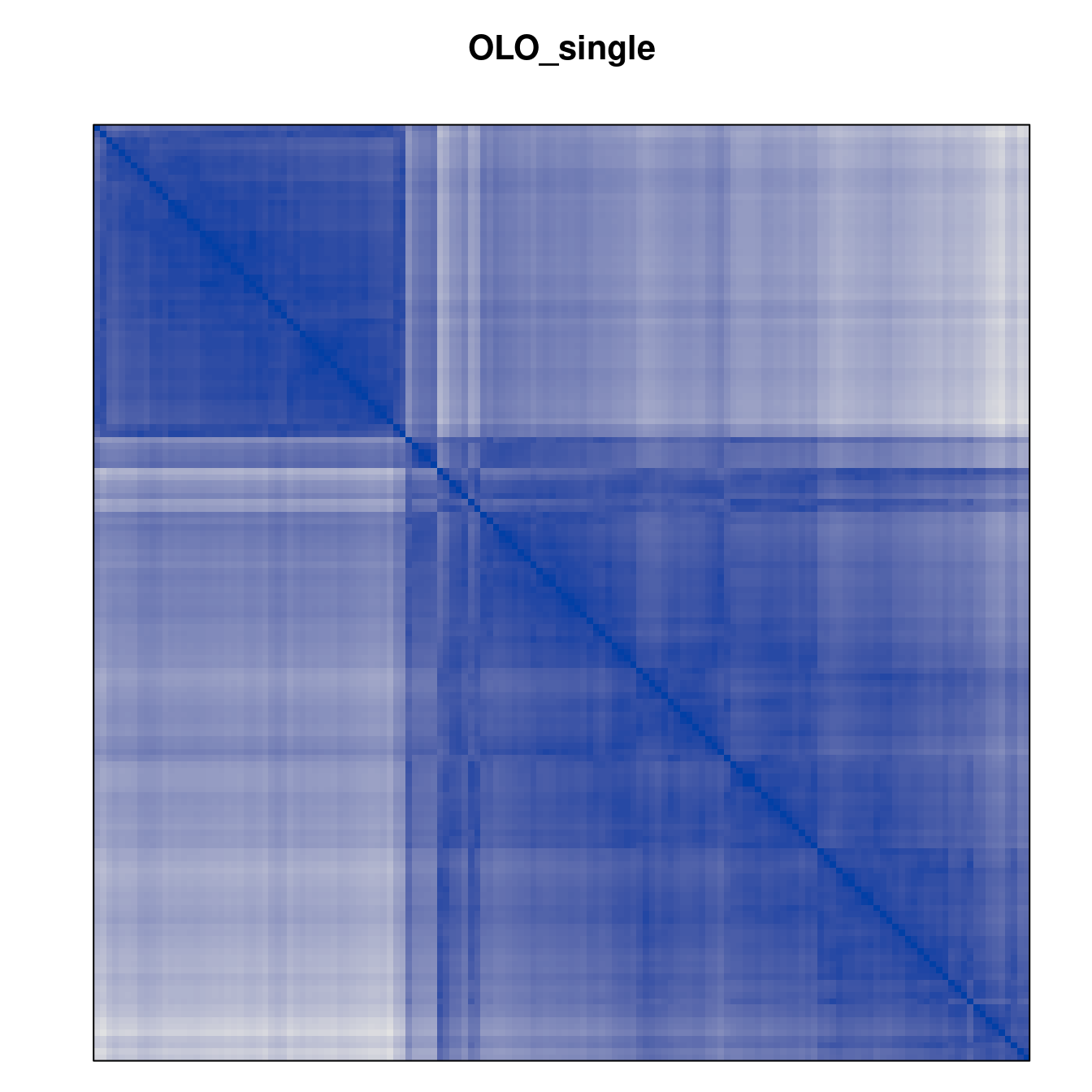
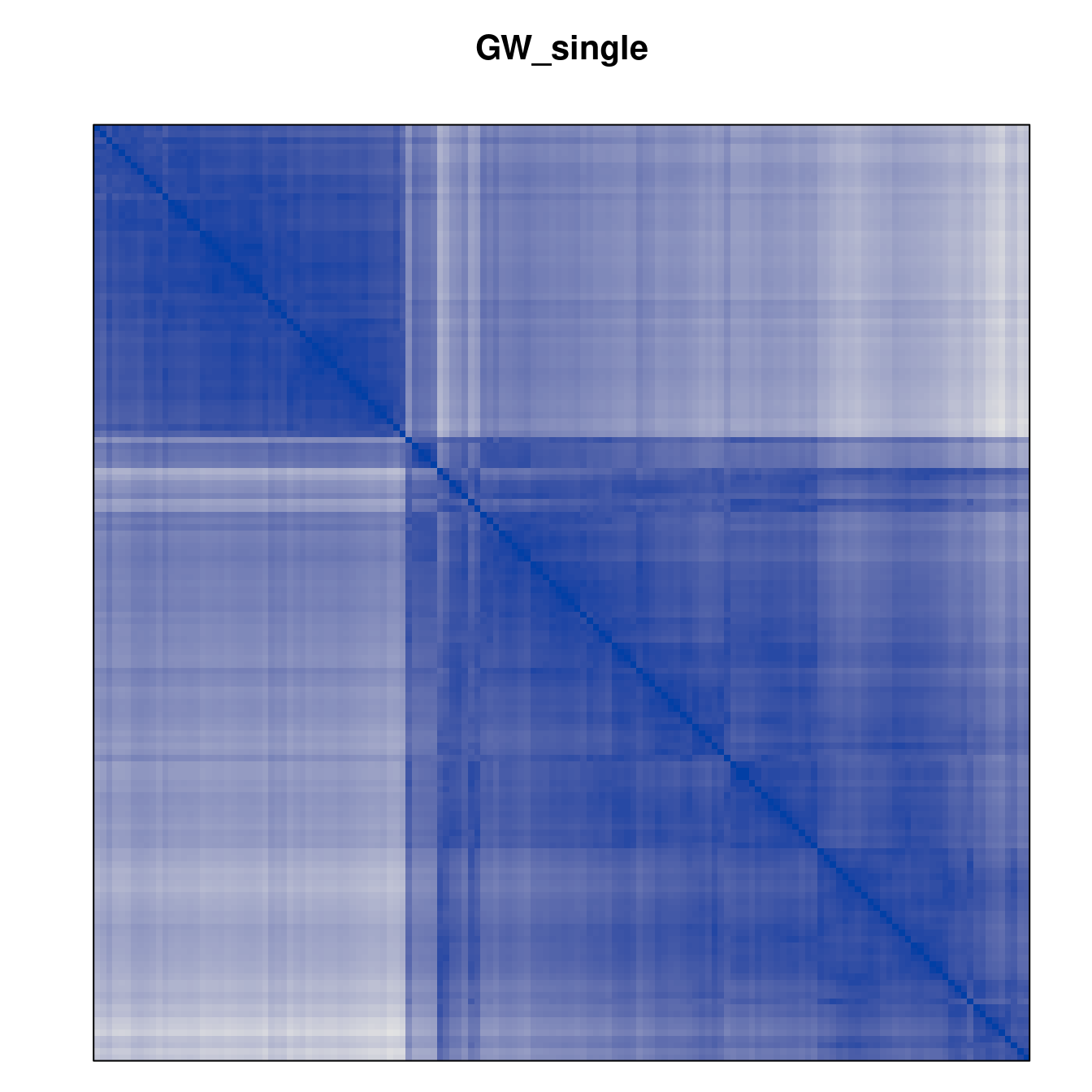
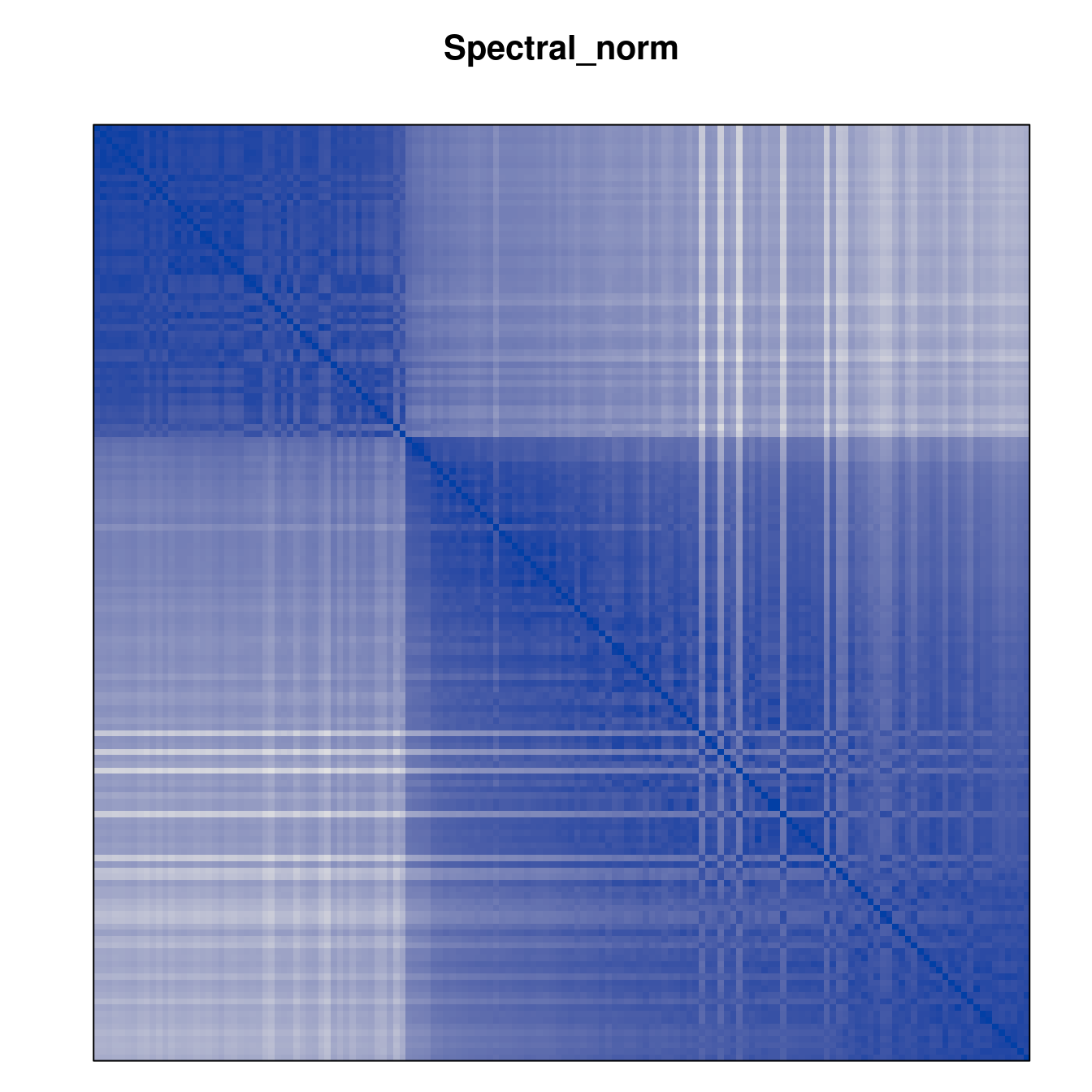
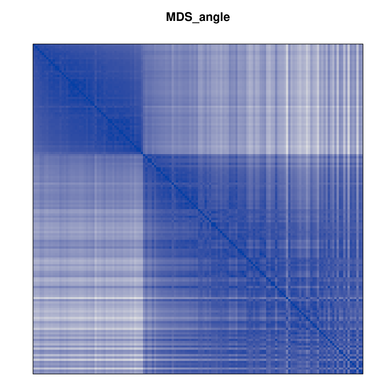
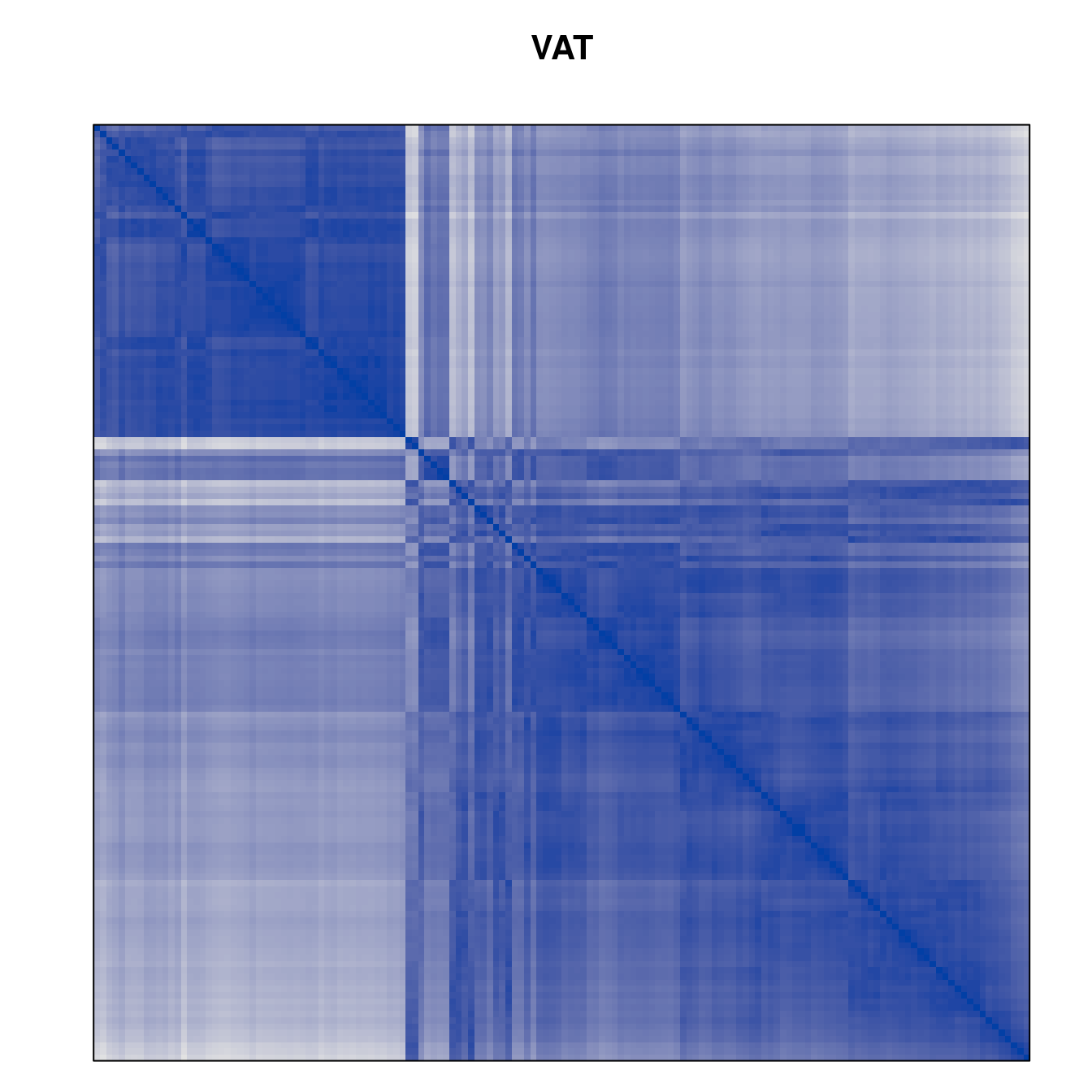
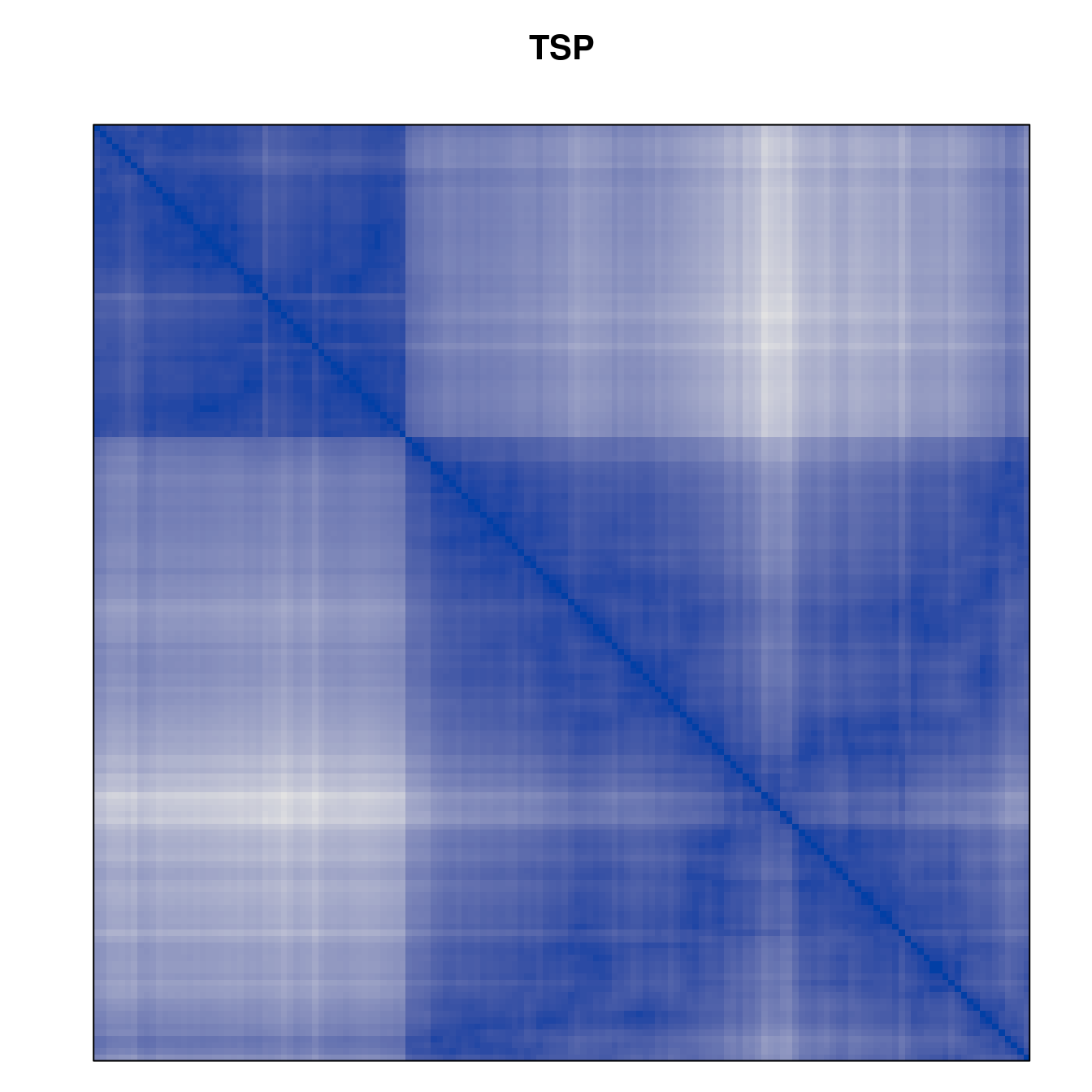
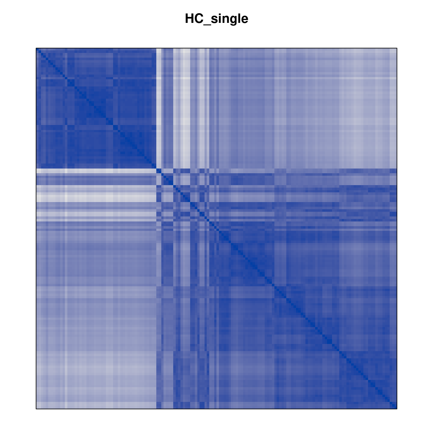
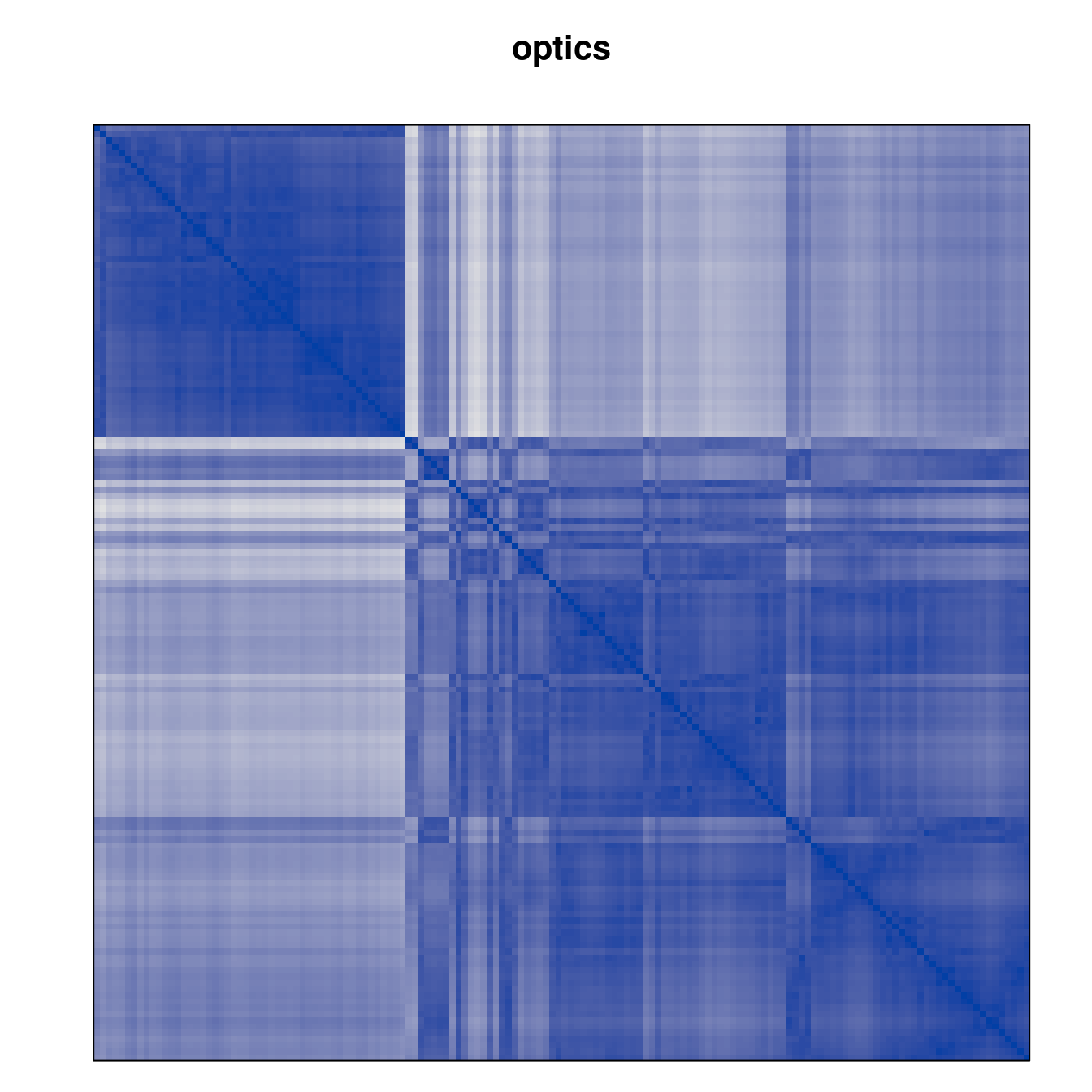
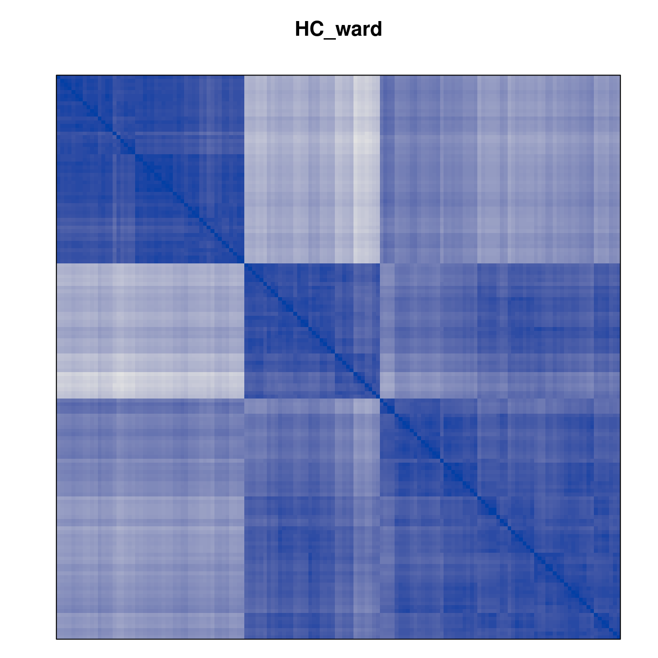
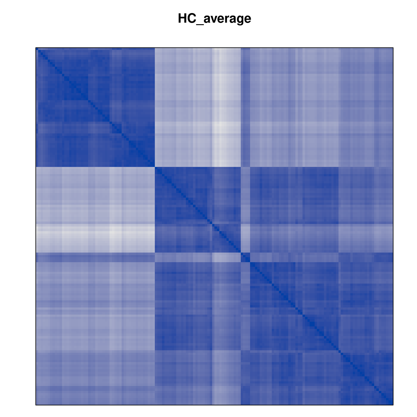
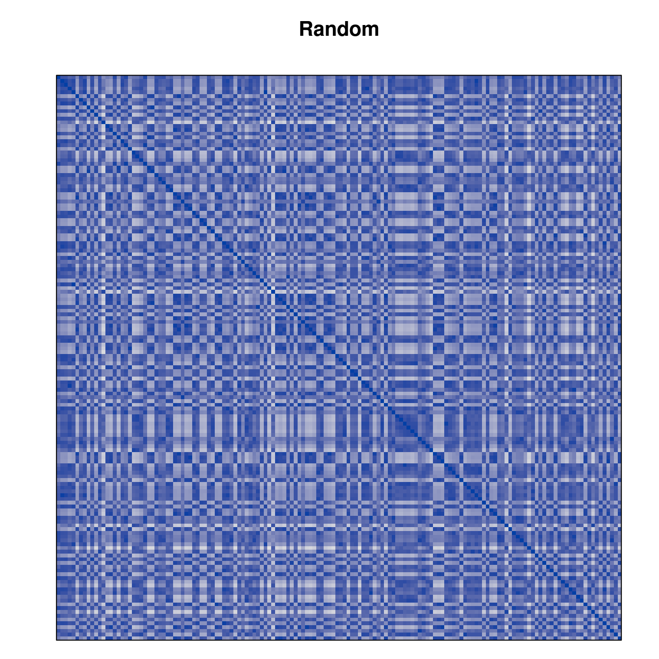
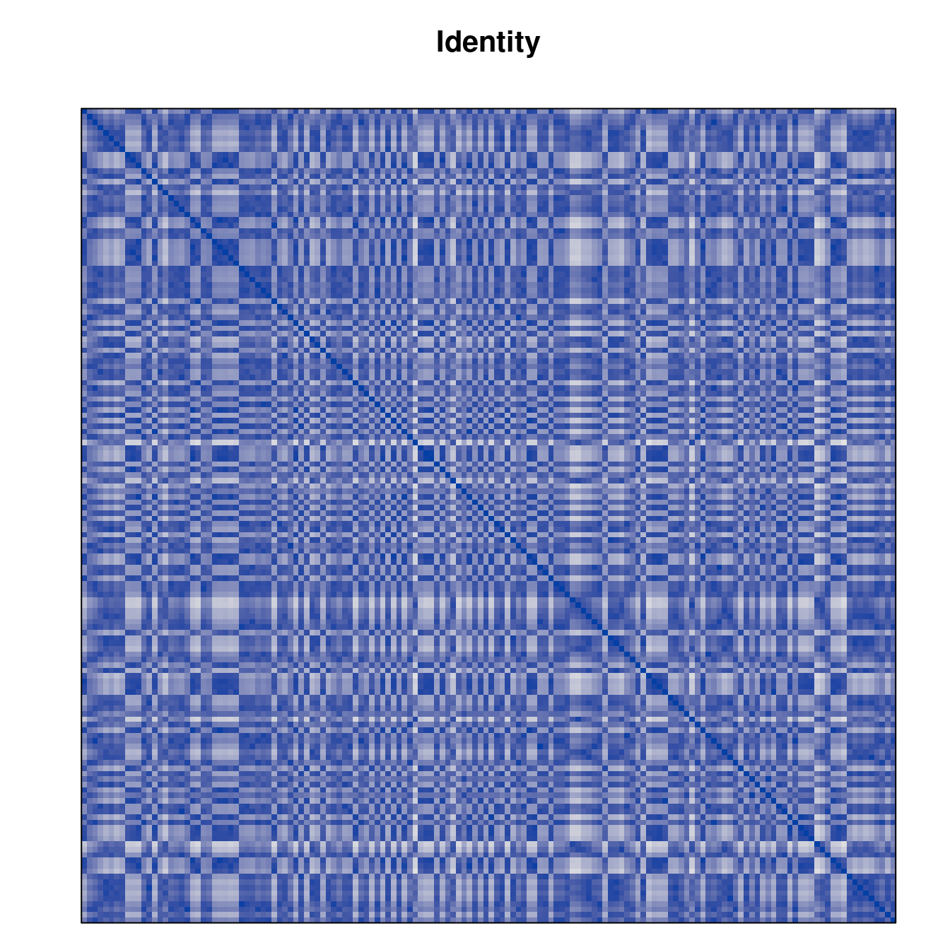
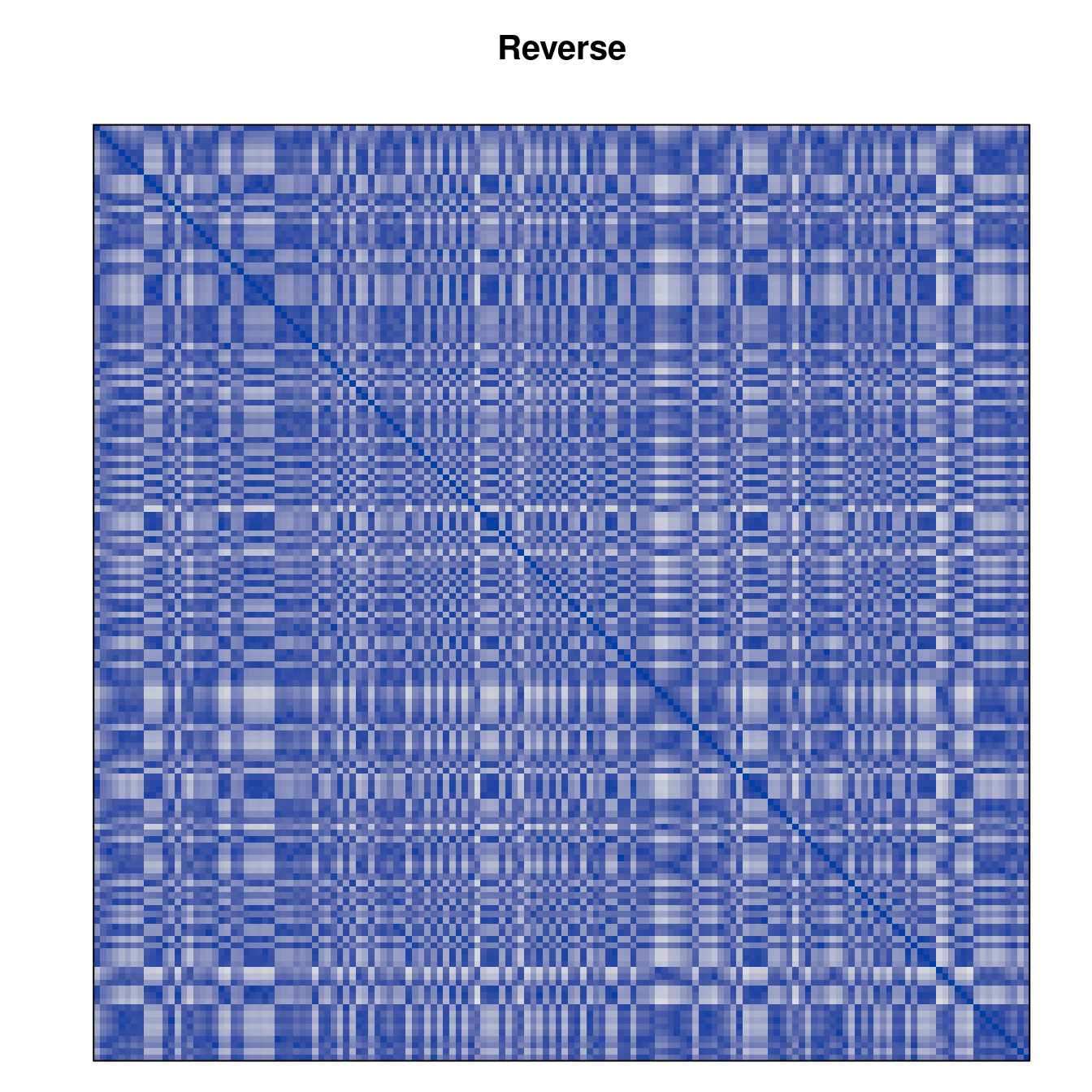
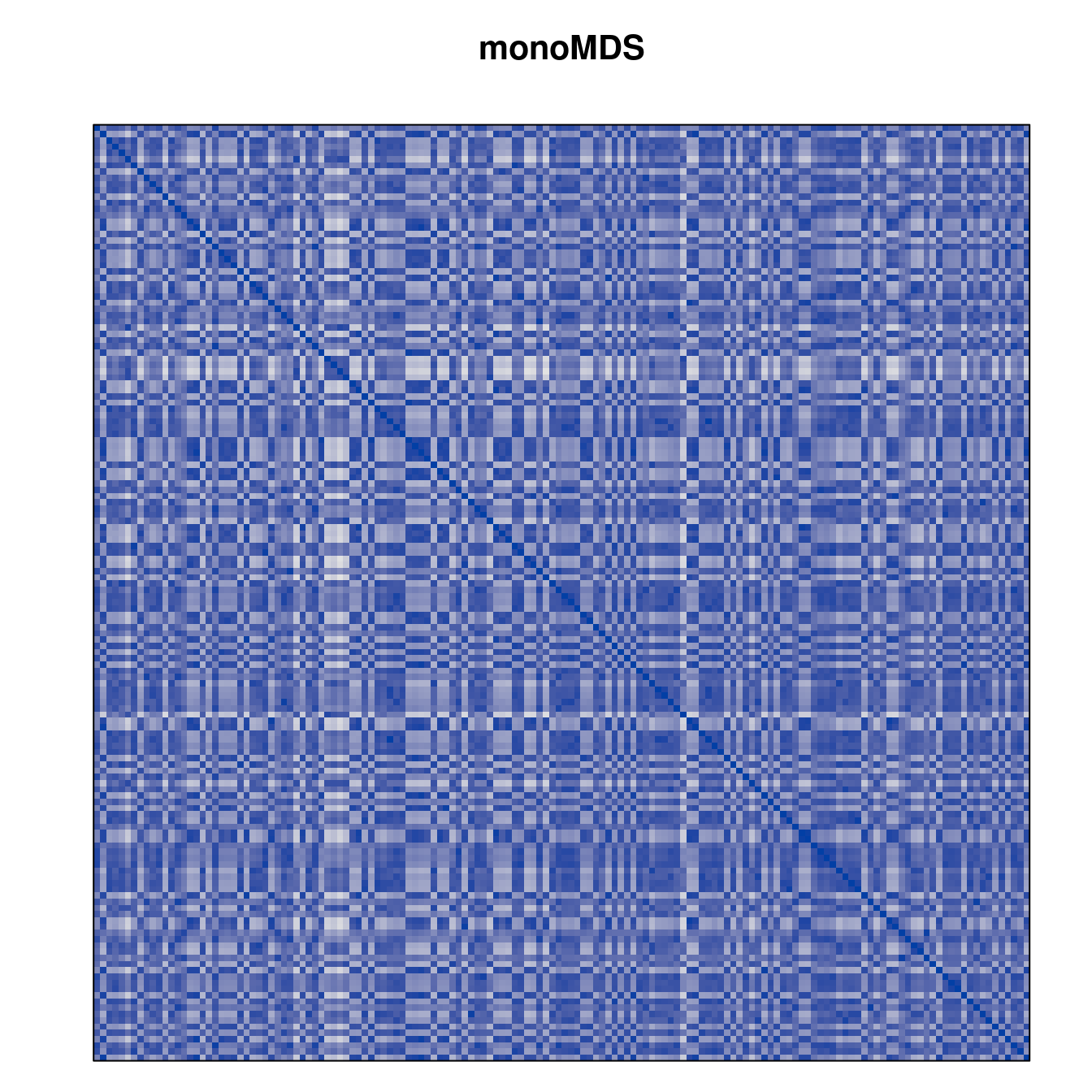
Plot the reordered dissimilarity matrices. Dark blocks along the main diagonal mean that the order reveals a “cluster” of similar objects. The Iris dataset contains three species, but two of them are very similar, so we expect to see one smaller block and one larger block.

for (n in names(orders))
  pimage(d, orders[[n]], main = n , key = FALSE)

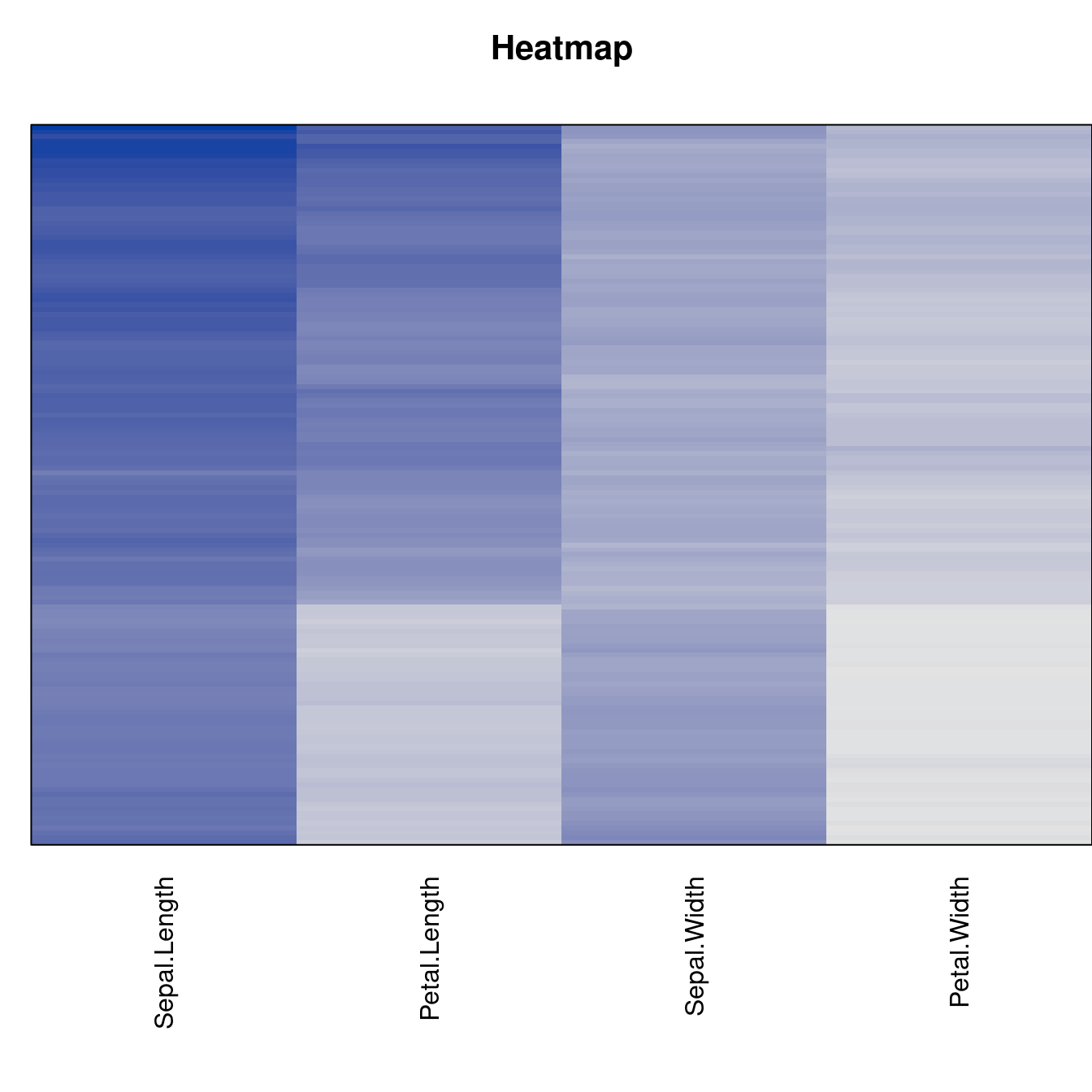
Matrix seriation

Matrix seriation reorders rows and columns of a data matrix. We perform the same steps as for distances in the previous section.

methods <- sort(list_seriation_methods("matrix"))

# AOE if for correlation matrices only
methods <- setdiff(methods, c("AOE"))
methods

 [1] "BEA"              "BEA_TSP"          "BK_unconstrained" "CA"              
 [5] "Heatmap"          "Identity"         "LLE"              "Mean"            
 [9] "PCA"              "PCA_angle"        "Random"           "Reverse"

Performing seriation.

orders <- list()
criterion <- list()
for (m in methods) {
  cat(m)
  tm <- system.time(orders[[m]] <- seriate(x, method = m))
  criterion[[m]] <- data.frame(time = tm[1]+tm[2], rbind(criterion(x, orders[[m]])))
  cat(" took", tm[1]+tm[2], "sec.\n")
}

BEA took 0.562 sec.
BEA_TSP took 0.511 sec.
BK_unconstrained took 0.171 sec.
CA took 0.167 sec.
Heatmap took 0.55 sec.
Identity took 0.17 sec.
LLE took 0.454 sec.
Mean took 0.167 sec.
PCA took 0.168 sec.
PCA_angle

Warning in prcomp.default(x, center = center, scale. = scale, rank = 2L):
partial argument match of 'rank' to 'rank.'

Warning in prcomp.default(t(x), center = center, scale. = scale, rank = 2L):
partial argument match of 'rank' to 'rank.'

 took 0.173 sec.
Random took 0.167 sec.
Reverse took 0.172 sec.

criterion <- do.call(rbind, criterion)

Comparison between methods

datatable(round(criterion, 2), extensions = "FixedColumns",
    options = list(paging = TRUE, searching = TRUE, info = FALSE,
      sort = TRUE, scrollX = TRUE, fixedColumns = list(leftColumns = 1))) %>%
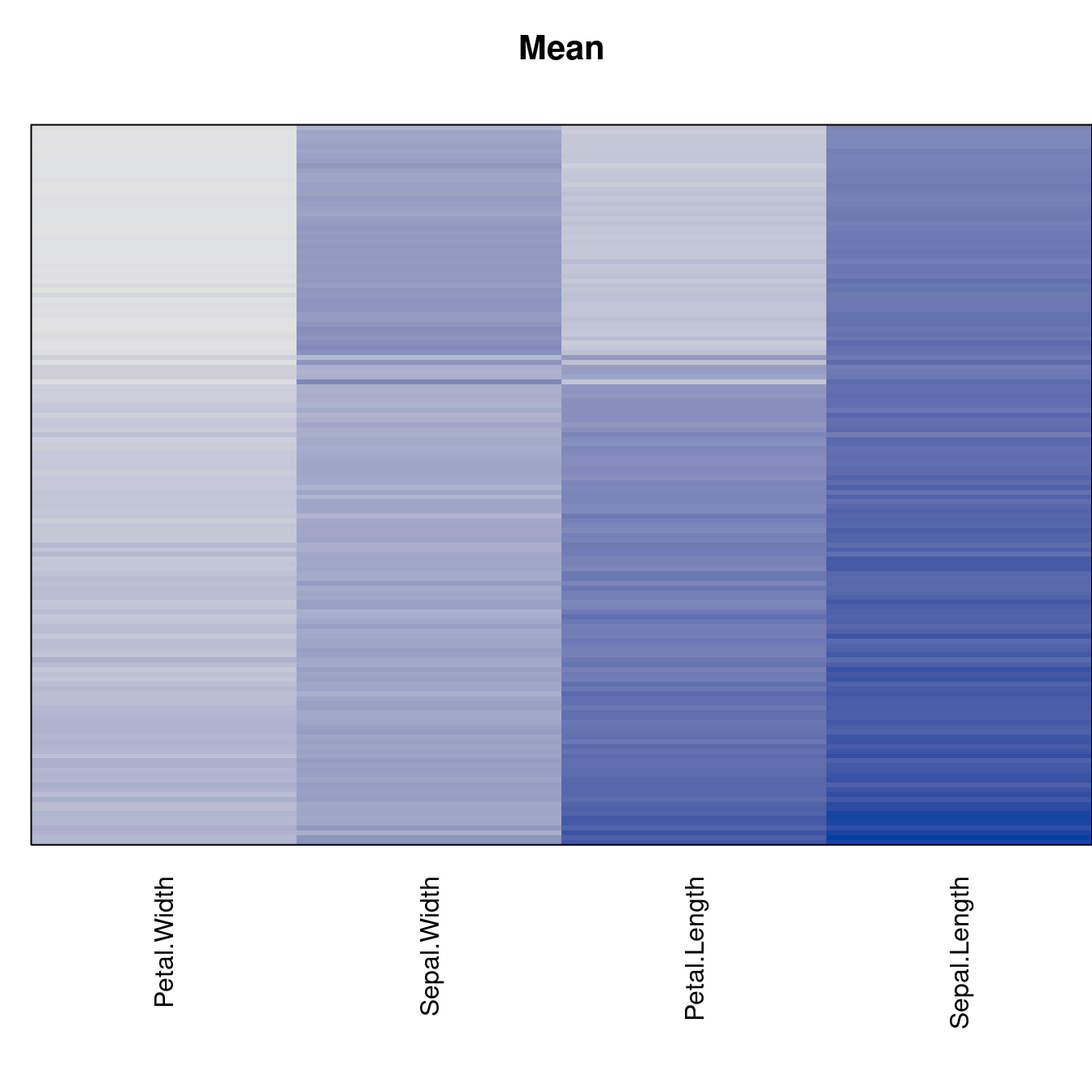
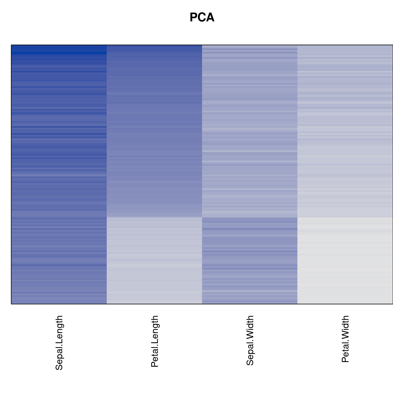
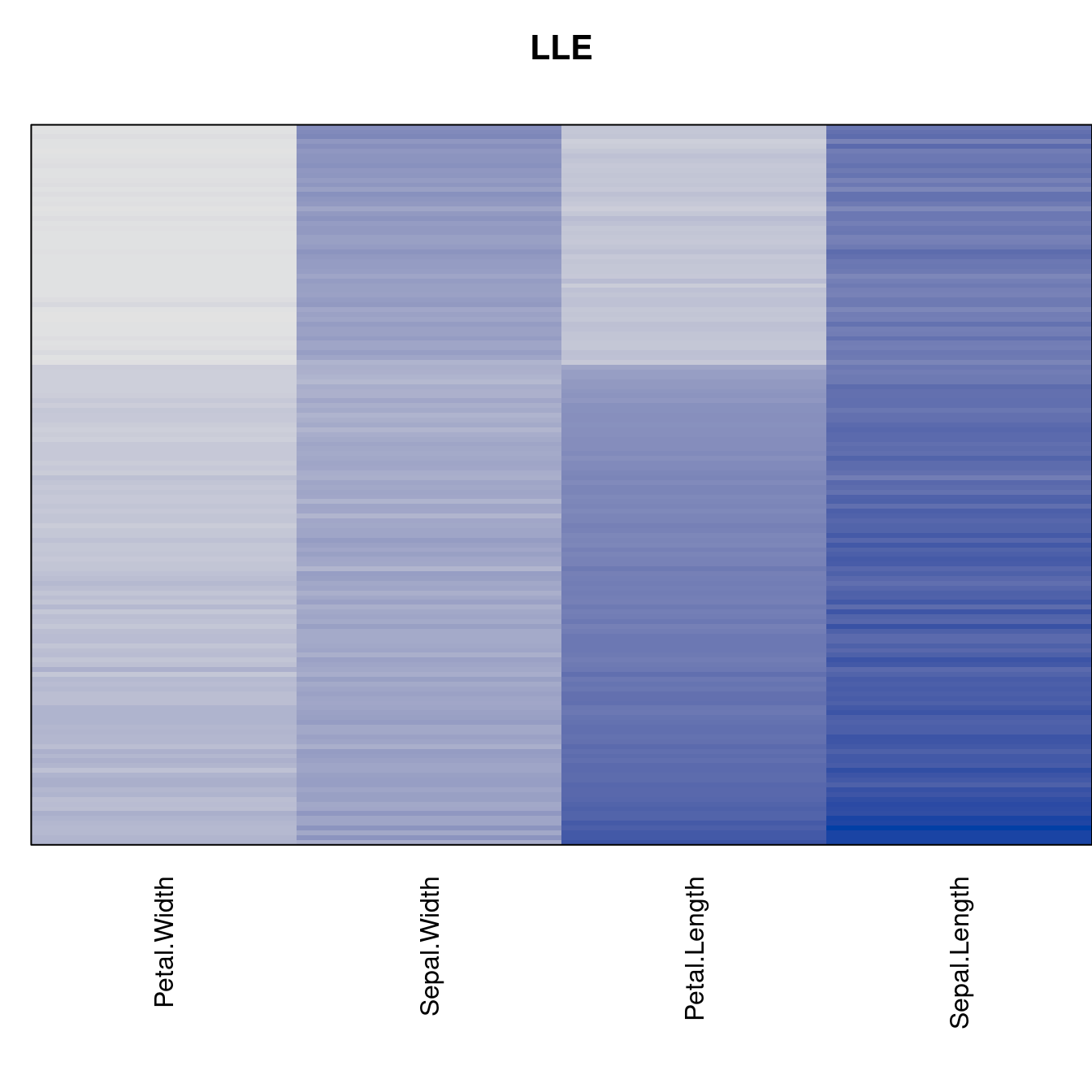
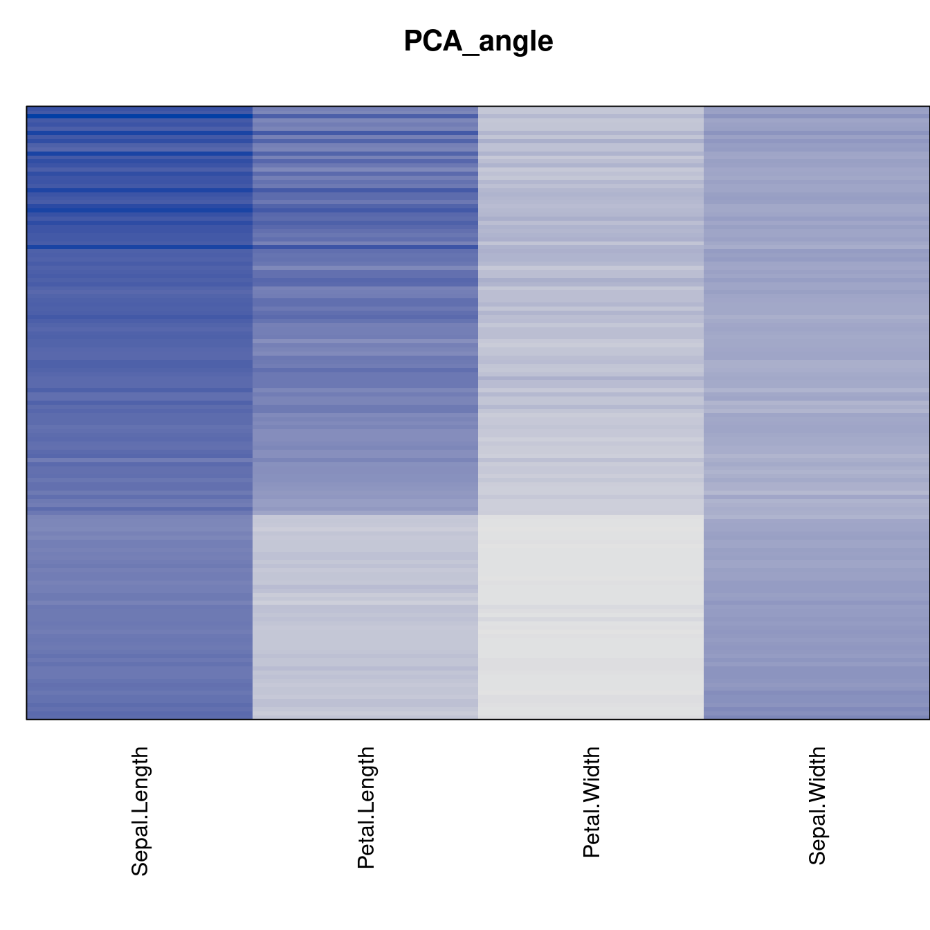
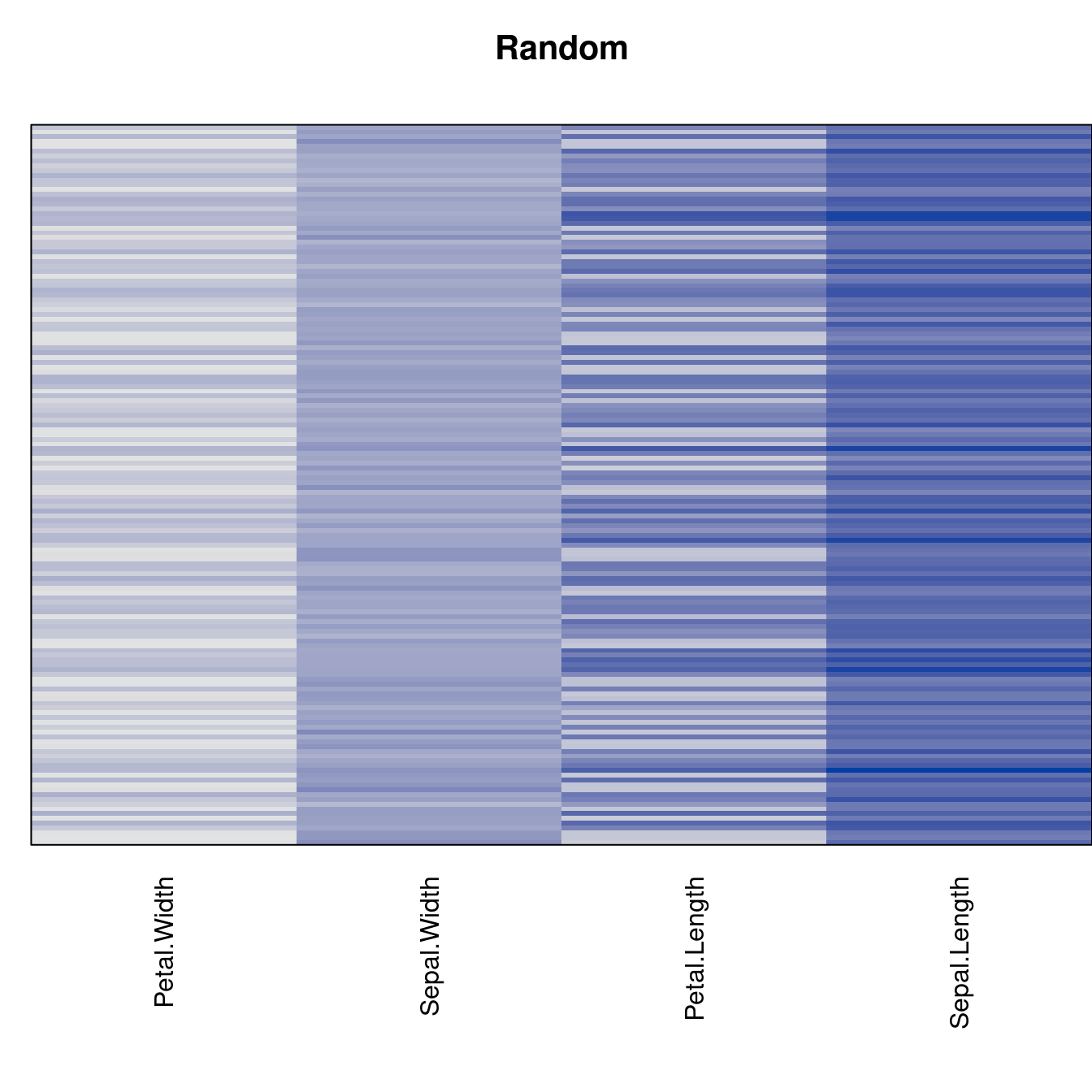
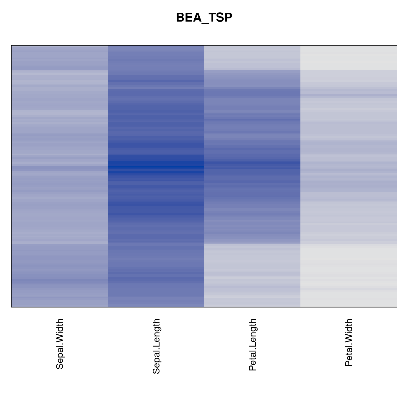
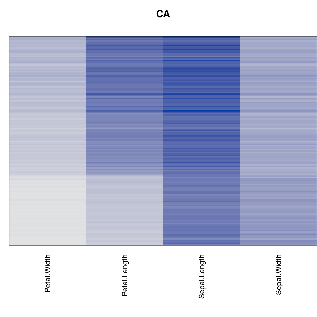
    formatRound(columns = colnames(criterion) , mark = "", digits = 1)

Visualize the results

best_to_worse <- order(criterion[["Moore_stress"]], decreasing = FALSE)

orders <- orders[best_to_worse]
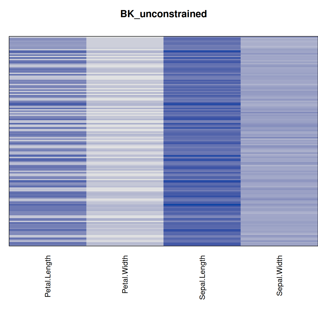
criterion <- criterion[best_to_worse, ]

for (n in names(orders))
  pimage(x, orders[[n]], main = n , key = FALSE)