How to use Tree-Penalized Path Length Criterion with Package seriation

Introduction

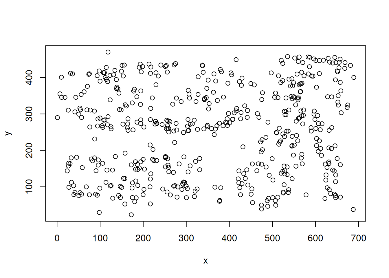
The tree-penalized path length criterion was introduced in

Denis A. Aliyev, Craig L. Zirbel, Seriation using tree-penalized path length, European Journal of Operational Research, Volume 305, Issue 2, 2023, Pages 617-629

This short vignette shows how to used tree-penalized path length criterion seriation with the R package seriation.

The idea of the tree-penalized path length criterion to use a TSP-based seriation on a modified distance matrix that adds clustering structure to the distance information. This is achieved by using the modified distance matrix:

\[T = D * \beta P\] where \(P\) contains the cophenetic distances for a hierarchical clustering. By adjusting \(\beta\), the seriation can be seamlessly move from a TSP based on only distances (\(\beta = 0\)) to a seriation order that represents purely the clustering structure (\(\beta = \infty\)).

Numeric Example

We use a sample of the Chameleon data set 7 which comes with the seriation package and has a cluster structure.

library("seriation")
data("Chameleon")

x <- chameleon_ds7[sample(1:nrow(chameleon_ds7), 500), ]
plot(x)

We calculate the penalty matrix from complete-link hierarchical clustering. The penalties are the copehenetic distances in the dendrogram.

D <- dist(x)

hc <- hclust(D, method = "complete")
plot(hc, labels = FALSE)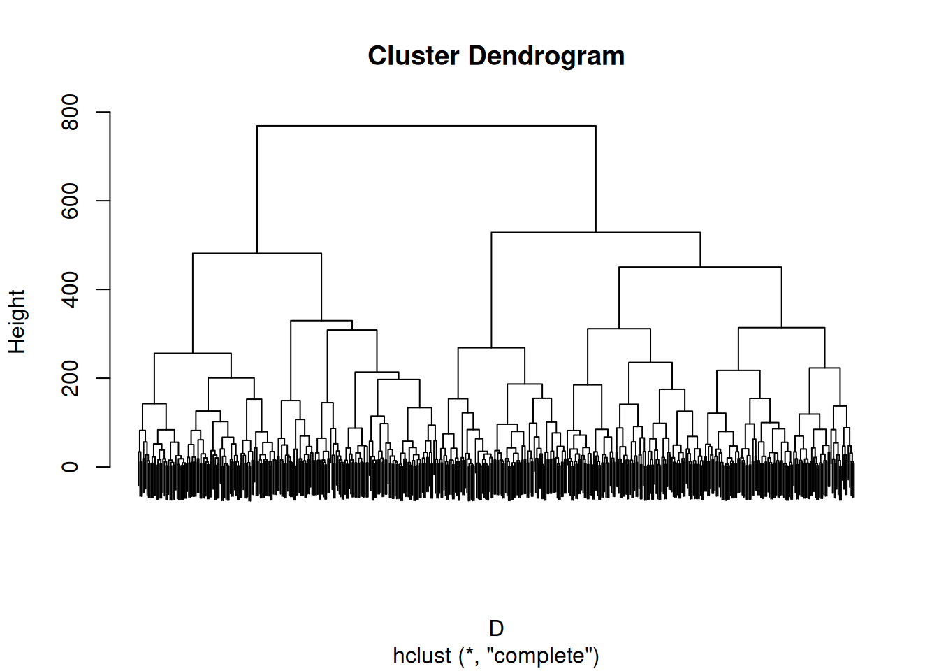

P <- cophenetic(hc)

Next, we calculate the penalized distance matrix, perform seriation and calculate the tree-penalized path length seriation criterion. The seriation criterion can be calculated using the path length criterion on the modified distance matrix \(F\).

beta <- 1
F <- D + beta * P

o <- seriate(F, method = "TSP")
criterion(F, o, method = "Path_length")

Path_length 
   28552.86 

Finally, we perform TSP seriation using different values for \(\beta\) to see how the clustering structure emerges more and more in the seriation result.

betas <- c(0, .25, .5, 1, 2, 10)

for (beta in betas) {
  F <- D + beta * P
  pimage(F, order = "TSP", main = paste("beta =", beta))
}

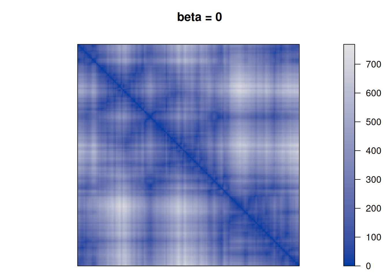
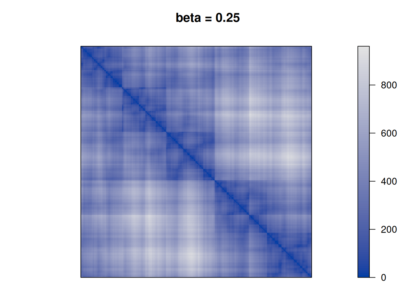
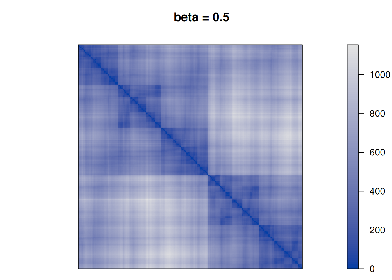
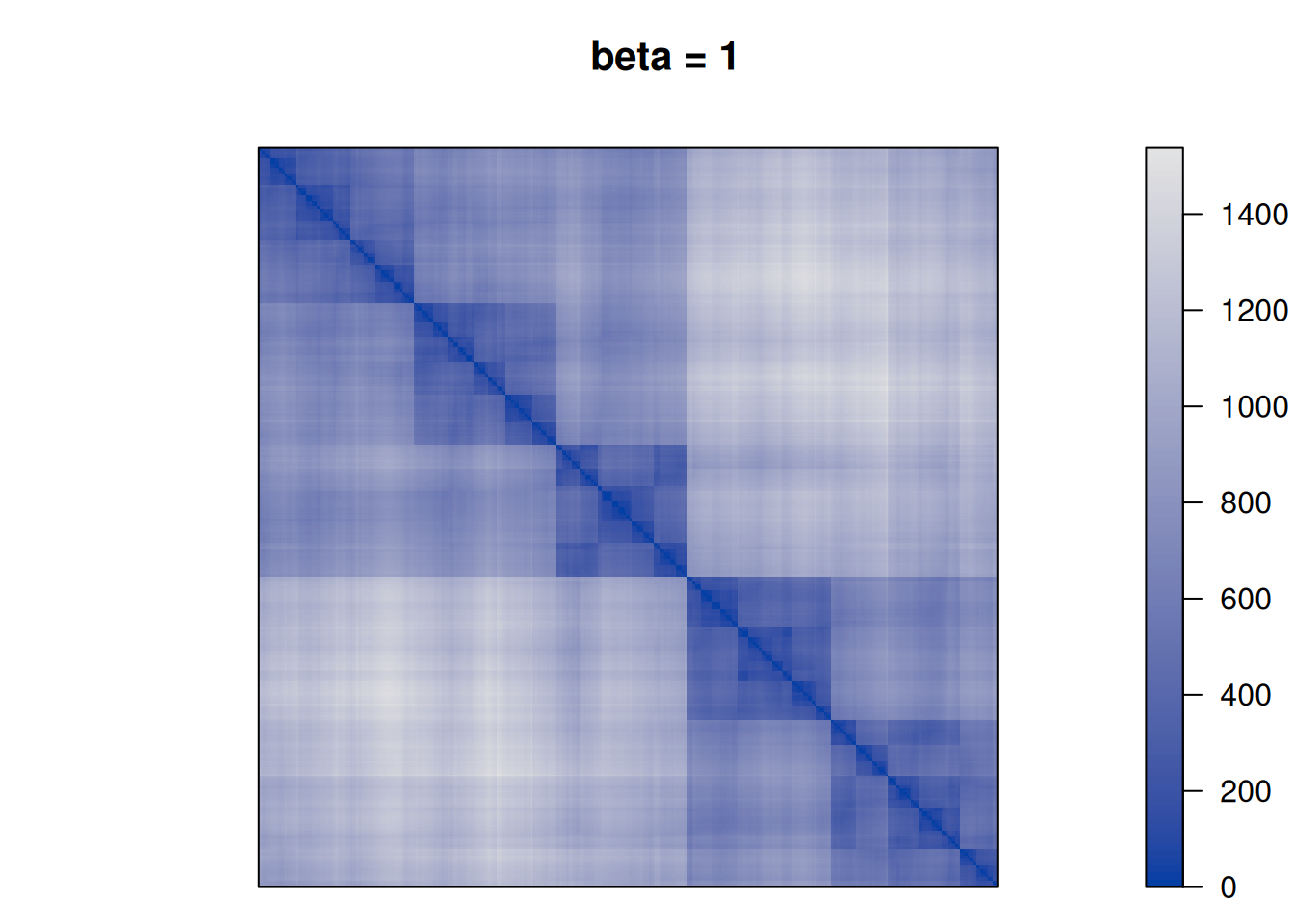
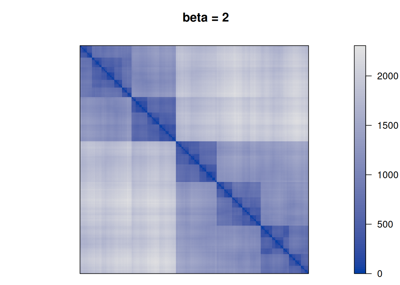
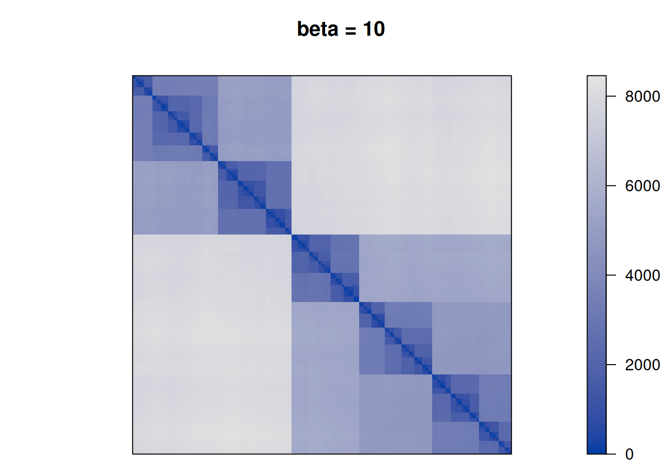
We see that as \(\beta\) is increased the seriation follows more and more the clustering. For \(\beta\) approaching \(\infty\), the seriation order approaches optimal leaf ordering (OLO).