5 Association Analysis: Basic Concepts and Algorithms
This chapter introduces association rules mining using the APRIORI algorithm. In addition, analyzing sets of association rules using visualization techniques is demonstrated.
The corresponding chapter of the data mining textbook is available online: Chapter 5: Association Analysis: Basic Concepts and Algorithms.
Packages Used in this Chapter
pkgs <- c("arules", "arulesViz", "mlbench", "palmerpenguins", "tidyverse")

pkgs_install <- pkgs[!(pkgs %in% installed.packages()[,"Package"])]
if(length(pkgs_install)) install.packages(pkgs_install)
The packages used for this chapter are: arules (Hahsler et al. 2024), arulesViz (Hahsler 2024), mlbench (Leisch and Dimitriadou 2024), palmerpenguins (Horst, Hill, and Gorman 2022), tidyverse (Wickham 2023c)
5.1 Preliminaries
Association rule mining plays a vital role in discovering hidden patterns and relationships within large transactional datasets. Applications range from exploratory data analysis in marketing to building rule-based classifiers. Agrawal, Imielinski, and Swami (1993) introduced the problem of mining association rules from transaction data as follows (the definition is taken from Hahsler, Grün, and Hornik (2005)):
Let \(I = \{i_1,i_2,...,i_n\}\) be a set of \(n\) binary attributes called items. Let \(D = \{t_1,t_2,...,t_m\}\) be a set of transactions called the database. Each transaction in \(D\) has a unique transaction ID and contains a subset of the items in \(I\). A rule is defined as an implication of the form \(X \Rightarrow Y\) where \(X,Y \subseteq I\) and \(X \cap Y = \emptyset\) are called itemsets. On itemsets and rules several quality measures can be defined. The most important measures are support and confidence. The support \(supp(X)\) of an itemset \(X\) is defined as the proportion of transactions in the data set which contain the itemset. Itemsets with a support which surpasses a user-defined threshold \(\sigma\) are called frequent itemsets. The confidence of a rule is defined as \(conf(X \Rightarrow Y) = supp(X \cup Y)/supp(X)\). Association rules are rules with \(supp(X \cup Y) \ge \sigma\) and \(conf(X) \ge \delta\) where \(\sigma\) and \(\delta\) are user-defined thresholds. The found set of association rules is then used reason about the data.
You can read the free sample chapter from the textbook (Tan, Steinbach, and Kumar 2005): Chapter 5. Association Analysis: Basic Concepts and Algorithms
5.1.1 The arules Package
Association rule mining in R is implemented in the package arules.
For information about the arules package try: help(package="arules")
and vignette("arules") (also available at
CRAN)
arules uses the S4 object system to implement classes and methods.
Standard R objects use the S3 object
system which do not use formal class
definitions and are usually implemented as a list with a class
attribute. arules and many other R packages use the S4 object
system which is based on formal class
definitions with member variables and methods (similar to
object-oriented programming languages like Java and C++). Some important
differences of using S4 objects compared to the usual S3 objects are:
- coercion (casting):
as(from, "class_name") - help for classes:
class? class_name
5.1.2 Transactions
5.1.2.1 Create Transactions
We will use the Zoo dataset from mlbench.
data(Zoo, package = "mlbench")
head(Zoo)
##           hair feathers  eggs  milk airborne aquatic predator toothed
## aardvark  TRUE    FALSE FALSE  TRUE    FALSE   FALSE     TRUE    TRUE
## antelope  TRUE    FALSE FALSE  TRUE    FALSE   FALSE    FALSE    TRUE
## bass     FALSE    FALSE  TRUE FALSE    FALSE    TRUE     TRUE    TRUE
## bear      TRUE    FALSE FALSE  TRUE    FALSE   FALSE     TRUE    TRUE
## boar      TRUE    FALSE FALSE  TRUE    FALSE   FALSE     TRUE    TRUE
## buffalo   TRUE    FALSE FALSE  TRUE    FALSE   FALSE    FALSE    TRUE
##          backbone breathes venomous  fins legs  tail domestic catsize
## aardvark     TRUE     TRUE    FALSE FALSE    4 FALSE    FALSE    TRUE
## antelope     TRUE     TRUE    FALSE FALSE    4  TRUE    FALSE    TRUE
## bass         TRUE    FALSE    FALSE  TRUE    0  TRUE    FALSE   FALSE
## bear         TRUE     TRUE    FALSE FALSE    4 FALSE    FALSE    TRUE
## boar         TRUE     TRUE    FALSE FALSE    4  TRUE    FALSE    TRUE
## buffalo      TRUE     TRUE    FALSE FALSE    4  TRUE    FALSE    TRUE
##            type
## aardvark mammal
## antelope mammal
## bass       fish
## bear     mammal
## boar     mammal
## buffalo  mammal
The data in the data.frame need to be converted into a set of
transactions where each row represents a transaction and each column is
translated into items. This is done using the constructor
transactions(). For the Zoo data set this means that we consider
animals as transactions and the different traits (features) will become
items that each animal has. For example the animal antelope has the
item hair in its transaction.
trans <- transactions(Zoo)
## Warning: Column(s) 13 not logical or factor. Applying default
## discretization (see '? discretizeDF').
The conversion gives a warning because only discrete features (factor
and logical) can be directly translated into items. Continuous
features need to be discretized first.
What is column 13?
summary(Zoo[13])
##       legs
##  Min.   :0.00
##  1st Qu.:2.00
##  Median :4.00
##  Mean   :2.84
##  3rd Qu.:4.00
##  Max.   :8.00
Zoo$legs |> table()
##
##  0  2  4  5  6  8
## 23 27 38  1 10  2
Possible solution: Make legs into has/does not have legs
Zoo_has_legs$legs |> table()
##
## FALSE  TRUE
##    23    78
Alternatives:
- use each unique value as an item:
Zoo_unique_leg_values <- Zoo |> mutate(legs = factor(legs))
Zoo_unique_leg_values$legs |> head()
## [1] 4 4 0 4 4 4
## Levels: 0 2 4 5 6 8- discretize (see
? discretizeand discretization in the code for Chapter 2):
Zoo_discretized_legs <- Zoo |> mutate(
  legs = discretize(legs, breaks = 2, method="interval")
)
table(Zoo_discretized_legs$legs)
##
## [0,4) [4,8]
##    50    51
Convert data into a set of transactions
trans <- transactions(Zoo_has_legs)
trans
## transactions in sparse format with
##  101 transactions (rows) and
##  23 items (columns)
5.1.2.2 Inspect Transactions
summary(trans)
## transactions as itemMatrix in sparse format with
##  101 rows (elements/itemsets/transactions) and
##  23 columns (items) and a density of 0.3612
##
## most frequent items:
## backbone breathes     legs     tail  toothed  (Other)
##       83       80       78       75       61      462
##
## element (itemset/transaction) length distribution:
## sizes
##  3  4  5  6  7  8  9 10 11 12
##  3  2  6  5  8 21 27 25  3  1
##
##    Min. 1st Qu.  Median    Mean 3rd Qu.    Max.
##    3.00    8.00    9.00    8.31   10.00   12.00
##
## includes extended item information - examples:
##     labels variables levels
## 1     hair      hair   TRUE
## 2 feathers  feathers   TRUE
## 3     eggs      eggs   TRUE
##
## includes extended transaction information - examples:
##   transactionID
## 1      aardvark
## 2      antelope
## 3          bass
Look at created items. They are still called column names since the transactions are actually stored as a large sparse logical matrix (see below).
colnames(trans)
##  [1] "hair"               "feathers"           "eggs"
##  [4] "milk"               "airborne"           "aquatic"
##  [7] "predator"           "toothed"            "backbone"
## [10] "breathes"           "venomous"           "fins"
## [13] "legs"               "tail"               "domestic"
## [16] "catsize"            "type=mammal"        "type=bird"
## [19] "type=reptile"       "type=fish"          "type=amphibian"
## [22] "type=insect"        "type=mollusc.et.al"
Compare with the original features (column names) from Zoo
colnames(Zoo)
##  [1] "hair"     "feathers" "eggs"     "milk"     "airborne" "aquatic"
##  [7] "predator" "toothed"  "backbone" "breathes" "venomous" "fins"
## [13] "legs"     "tail"     "domestic" "catsize"  "type"
Look at a (first) few transactions as a matrix. 1 indicates the presence of an item.
as(trans, "matrix")[1:3,]
##           hair feathers  eggs  milk airborne aquatic predator toothed
## aardvark  TRUE    FALSE FALSE  TRUE    FALSE   FALSE     TRUE    TRUE
## antelope  TRUE    FALSE FALSE  TRUE    FALSE   FALSE    FALSE    TRUE
## bass     FALSE    FALSE  TRUE FALSE    FALSE    TRUE     TRUE    TRUE
##          backbone breathes venomous  fins  legs  tail domestic
## aardvark     TRUE     TRUE    FALSE FALSE  TRUE FALSE    FALSE
## antelope     TRUE     TRUE    FALSE FALSE  TRUE  TRUE    FALSE
## bass         TRUE    FALSE    FALSE  TRUE FALSE  TRUE    FALSE
##          catsize type=mammal type=bird type=reptile type=fish
## aardvark    TRUE        TRUE     FALSE        FALSE     FALSE
## antelope    TRUE        TRUE     FALSE        FALSE     FALSE
## bass       FALSE       FALSE     FALSE        FALSE      TRUE
##          type=amphibian type=insect type=mollusc.et.al
## aardvark          FALSE       FALSE              FALSE
## antelope          FALSE       FALSE              FALSE
## bass              FALSE       FALSE              FALSE
Look at the transactions as sets of items
inspect(trans[1:3])
##     items         transactionID
## [1] {hair,
##      milk,
##      predator,
##      toothed,
##      backbone,
##      breathes,
##      legs,
##      catsize,
##      type=mammal}      aardvark
## [2] {hair,
##      milk,
##      toothed,
##      backbone,
##      breathes,
##      legs,
##      tail,
##      catsize,
##      type=mammal}      antelope
## [3] {eggs,
##      aquatic,
##      predator,
##      toothed,
##      backbone,
##      fins,
##      tail,
##      type=fish}        bass
Plot the binary matrix. Dark dots represent 1s.
image(trans)
Look at the relative frequency (=support) of items in the data set. Here we look at the 10 most frequent items.
itemFrequencyPlot(trans,topN = 20)
ggplot(
  tibble(
    Support = sort(itemFrequency(trans, type = "absolute"), decreasing = TRUE),
    Item = seq_len(ncol(trans))
  ), aes(x = Item, y = Support)) + geom_line()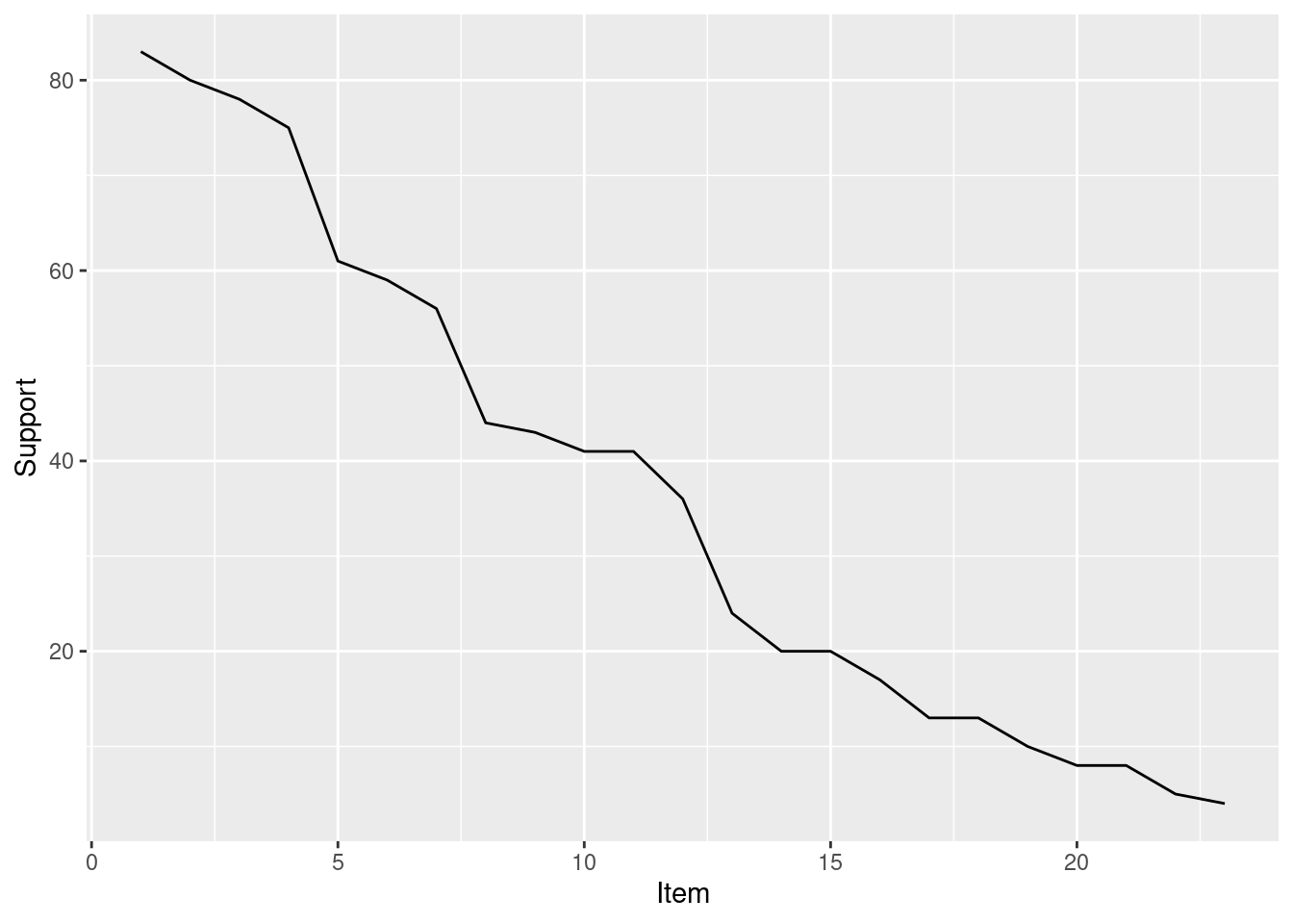
Alternative encoding: Also create items for FALSE (use factor)
sapply(Zoo_has_legs, class)
##      hair  feathers      eggs      milk  airborne   aquatic  predator
## "logical" "logical" "logical" "logical" "logical" "logical" "logical"
##   toothed  backbone  breathes  venomous      fins      legs      tail
## "logical" "logical" "logical" "logical" "logical" "logical" "logical"
##  domestic   catsize      type
## "logical" "logical"  "factor"
Zoo_factors <- Zoo_has_legs |> mutate(across(where(is.logical), factor))
sapply(Zoo_factors, class)
##     hair feathers     eggs     milk airborne  aquatic predator
## "factor" "factor" "factor" "factor" "factor" "factor" "factor"
##  toothed backbone breathes venomous     fins     legs     tail
## "factor" "factor" "factor" "factor" "factor" "factor" "factor"
## domestic  catsize     type
## "factor" "factor" "factor"
summary(Zoo_factors)
##     hair     feathers     eggs       milk     airborne   aquatic
##  FALSE:58   FALSE:81   FALSE:42   FALSE:60   FALSE:77   FALSE:65
##  TRUE :43   TRUE :20   TRUE :59   TRUE :41   TRUE :24   TRUE :36
##
##
##
##
##
##   predator   toothed    backbone   breathes   venomous     fins
##  FALSE:45   FALSE:40   FALSE:18   FALSE:21   FALSE:93   FALSE:84
##  TRUE :56   TRUE :61   TRUE :83   TRUE :80   TRUE : 8   TRUE :17
##
##
##
##
##
##     legs       tail     domestic   catsize              type
##  FALSE:23   FALSE:26   FALSE:88   FALSE:57   mammal       :41
##  TRUE :78   TRUE :75   TRUE :13   TRUE :44   bird         :20
##                                              reptile      : 5
##                                              fish         :13
##                                              amphibian    : 4
##                                              insect       : 8
##                                              mollusc.et.al:10
trans_factors <- transactions(Zoo_factors)
trans_factors
## transactions in sparse format with
##  101 transactions (rows) and
##  39 items (columns)
itemFrequencyPlot(trans_factors, topN = 20)
## Select transactions that contain a certain item
trans_insects <- trans_factors[trans %in% "type=insect"]
trans_insects
## transactions in sparse format with
##  8 transactions (rows) and
##  39 items (columns)
inspect(trans_insects)
##     items             transactionID
## [1] {hair=FALSE,
##      feathers=FALSE,
##      eggs=TRUE,
##      milk=FALSE,
##      airborne=FALSE,
##      aquatic=FALSE,
##      predator=FALSE,
##      toothed=FALSE,
##      backbone=FALSE,
##      breathes=TRUE,
##      venomous=FALSE,
##      fins=FALSE,
##      legs=TRUE,
##      tail=FALSE,
##      domestic=FALSE,
##      catsize=FALSE,
##      type=insect}          flea
## [2] {hair=FALSE,
##      feathers=FALSE,
##      eggs=TRUE,
##      milk=FALSE,
##      airborne=TRUE,
##      aquatic=FALSE,
##      predator=FALSE,
##      toothed=FALSE,
##      backbone=FALSE,
##      breathes=TRUE,
##      venomous=FALSE,
##      fins=FALSE,
##      legs=TRUE,
##      tail=FALSE,
##      domestic=FALSE,
##      catsize=FALSE,
##      type=insect}          gnat
## [3] {hair=TRUE,
##      feathers=FALSE,
##      eggs=TRUE,
##      milk=FALSE,
##      airborne=TRUE,
##      aquatic=FALSE,
##      predator=FALSE,
##      toothed=FALSE,
##      backbone=FALSE,
##      breathes=TRUE,
##      venomous=TRUE,
##      fins=FALSE,
##      legs=TRUE,
##      tail=FALSE,
##      domestic=TRUE,
##      catsize=FALSE,
##      type=insect}          honeybee
## [4] {hair=TRUE,
##      feathers=FALSE,
##      eggs=TRUE,
##      milk=FALSE,
##      airborne=TRUE,
##      aquatic=FALSE,
##      predator=FALSE,
##      toothed=FALSE,
##      backbone=FALSE,
##      breathes=TRUE,
##      venomous=FALSE,
##      fins=FALSE,
##      legs=TRUE,
##      tail=FALSE,
##      domestic=FALSE,
##      catsize=FALSE,
##      type=insect}          housefly
## [5] {hair=FALSE,
##      feathers=FALSE,
##      eggs=TRUE,
##      milk=FALSE,
##      airborne=TRUE,
##      aquatic=FALSE,
##      predator=TRUE,
##      toothed=FALSE,
##      backbone=FALSE,
##      breathes=TRUE,
##      venomous=FALSE,
##      fins=FALSE,
##      legs=TRUE,
##      tail=FALSE,
##      domestic=FALSE,
##      catsize=FALSE,
##      type=insect}          ladybird
## [6] {hair=TRUE,
##      feathers=FALSE,
##      eggs=TRUE,
##      milk=FALSE,
##      airborne=TRUE,
##      aquatic=FALSE,
##      predator=FALSE,
##      toothed=FALSE,
##      backbone=FALSE,
##      breathes=TRUE,
##      venomous=FALSE,
##      fins=FALSE,
##      legs=TRUE,
##      tail=FALSE,
##      domestic=FALSE,
##      catsize=FALSE,
##      type=insect}          moth
## [7] {hair=FALSE,
##      feathers=FALSE,
##      eggs=TRUE,
##      milk=FALSE,
##      airborne=FALSE,
##      aquatic=FALSE,
##      predator=FALSE,
##      toothed=FALSE,
##      backbone=FALSE,
##      breathes=TRUE,
##      venomous=FALSE,
##      fins=FALSE,
##      legs=TRUE,
##      tail=FALSE,
##      domestic=FALSE,
##      catsize=FALSE,
##      type=insect}          termite
## [8] {hair=TRUE,
##      feathers=FALSE,
##      eggs=TRUE,
##      milk=FALSE,
##      airborne=TRUE,
##      aquatic=FALSE,
##      predator=FALSE,
##      toothed=FALSE,
##      backbone=FALSE,
##      breathes=TRUE,
##      venomous=TRUE,
##      fins=FALSE,
##      legs=TRUE,
##      tail=FALSE,
##      domestic=FALSE,
##      catsize=FALSE,
##      type=insect}          wasp
5.1.2.3 Vertical Layout (Transaction ID Lists)
The default layout for transactions is horizontal layout (i.e. each transaction is a row). The vertical layout represents transaction data as a list of transaction IDs for each item (= transaction ID lists).
vertical <- as(trans, "tidLists")
as(vertical, "matrix")[1:10, 1:5]
##          aardvark antelope  bass  bear  boar
## hair         TRUE     TRUE FALSE  TRUE  TRUE
## feathers    FALSE    FALSE FALSE FALSE FALSE
## eggs        FALSE    FALSE  TRUE FALSE FALSE
## milk         TRUE     TRUE FALSE  TRUE  TRUE
## airborne    FALSE    FALSE FALSE FALSE FALSE
## aquatic     FALSE    FALSE  TRUE FALSE FALSE
## predator     TRUE    FALSE  TRUE  TRUE  TRUE
## toothed      TRUE     TRUE  TRUE  TRUE  TRUE
## backbone     TRUE     TRUE  TRUE  TRUE  TRUE
## breathes     TRUE     TRUE FALSE  TRUE  TRUE
5.2 Frequent Itemset Generation
For this dataset we have already a huge number of possible itemsets
2^ncol(trans)
## [1] 8388608
Find frequent itemsets (target=“frequent”) with the default settings.
its <- apriori(trans, parameter=list(target = "frequent"))
## Apriori
##
## Parameter specification:
##  confidence minval smax arem  aval originalSupport maxtime support
##          NA    0.1    1 none FALSE            TRUE       5     0.1
##  minlen maxlen            target  ext
##       1     10 frequent itemsets TRUE
##
## Algorithmic control:
##  filter tree heap memopt load sort verbose
##     0.1 TRUE TRUE  FALSE TRUE    2    TRUE
##
## Absolute minimum support count: 10
##
## set item appearances ...[0 item(s)] done [0.00s].
## set transactions ...[23 item(s), 101 transaction(s)] done [0.00s].
## sorting and recoding items ... [18 item(s)] done [0.00s].
## creating transaction tree ... done [0.00s].
## checking subsets of size 1 2 3 4 5 6 7 8 9 10
## Warning in apriori(trans, parameter = list(target = "frequent")):
## Mining stopped (maxlen reached). Only patterns up to a length of 10
## returned!
##  done [0.00s].
## sorting transactions ... done [0.00s].
## writing ... [1465 set(s)] done [0.00s].
## creating S4 object  ... done [0.00s].
its
## set of 1465 itemsets
Default minimum support is .1 (10%). Note: We use here a very small data set. For larger datasets the default minimum support might be to low and you may run out of memory. You probably want to start out with a higher minimum support like .5 (50%) and then work your way down.
5/nrow(trans)
## [1] 0.0495
In order to find itemsets that effect 5 animals I need to go down to a support of about 5%.
its <- apriori(trans, parameter=list(target = "frequent", support = 0.05))
## Apriori
##
## Parameter specification:
##  confidence minval smax arem  aval originalSupport maxtime support
##          NA    0.1    1 none FALSE            TRUE       5    0.05
##  minlen maxlen            target  ext
##       1     10 frequent itemsets TRUE
##
## Algorithmic control:
##  filter tree heap memopt load sort verbose
##     0.1 TRUE TRUE  FALSE TRUE    2    TRUE
##
## Absolute minimum support count: 5
##
## set item appearances ...[0 item(s)] done [0.00s].
## set transactions ...[23 item(s), 101 transaction(s)] done [0.00s].
## sorting and recoding items ... [21 item(s)] done [0.00s].
## creating transaction tree ... done [0.00s].
## checking subsets of size 1 2 3 4 5 6 7 8 9 10
## Warning in apriori(trans, parameter = list(target = "frequent",
## support = 0.05)): Mining stopped (maxlen reached). Only patterns up
## to a length of 10 returned!
##  done [0.00s].
## sorting transactions ... done [0.00s].
## writing ... [2537 set(s)] done [0.00s].
## creating S4 object  ... done [0.00s].
its
## set of 2537 itemsets
Sort by support
its <- sort(its, by = "support")
its |> head(n = 10) |> inspect()
##      items                      support count
## [1]  {backbone}                 0.8218  83
## [2]  {breathes}                 0.7921  80
## [3]  {legs}                     0.7723  78
## [4]  {tail}                     0.7426  75
## [5]  {backbone, tail}           0.7327  74
## [6]  {breathes, legs}           0.7228  73
## [7]  {backbone, breathes}       0.6832  69
## [8]  {backbone, legs}           0.6337  64
## [9]  {backbone, breathes, legs} 0.6337  64
## [10] {toothed}                  0.6040  61
Look at frequent itemsets with many items (set breaks manually since Automatically chosen breaks look bad)
its[size(its) > 8] |> inspect()
##      items         support count
## [1]  {hair,
##       milk,
##       toothed,
##       backbone,
##       breathes,
##       legs,
##       tail,
##       catsize,
##       type=mammal} 0.23762    24
## [2]  {hair,
##       milk,
##       predator,
##       toothed,
##       backbone,
##       breathes,
##       legs,
##       catsize,
##       type=mammal} 0.15842    16
## [3]  {hair,
##       milk,
##       predator,
##       toothed,
##       backbone,
##       breathes,
##       legs,
##       tail,
##       type=mammal} 0.14851    15
## [4]  {hair,
##       milk,
##       predator,
##       backbone,
##       breathes,
##       legs,
##       tail,
##       catsize,
##       type=mammal} 0.13861    14
## [5]  {hair,
##       milk,
##       predator,
##       toothed,
##       breathes,
##       legs,
##       tail,
##       catsize,
##       type=mammal} 0.12871    13
## [6]  {hair,
##       milk,
##       predator,
##       toothed,
##       backbone,
##       legs,
##       tail,
##       catsize,
##       type=mammal} 0.12871    13
## [7]  {hair,
##       milk,
##       predator,
##       toothed,
##       backbone,
##       breathes,
##       tail,
##       catsize,
##       type=mammal} 0.12871    13
## [8]  {milk,
##       predator,
##       toothed,
##       backbone,
##       breathes,
##       legs,
##       tail,
##       catsize,
##       type=mammal} 0.12871    13
## [9]  {hair,
##       milk,
##       predator,
##       toothed,
##       backbone,
##       breathes,
##       legs,
##       tail,
##       catsize}     0.12871    13
## [10] {hair,
##       predator,
##       toothed,
##       backbone,
##       breathes,
##       legs,
##       tail,
##       catsize,
##       type=mammal} 0.12871    13
## [11] {hair,
##       milk,
##       predator,
##       toothed,
##       backbone,
##       breathes,
##       legs,
##       tail,
##       catsize,
##       type=mammal} 0.12871    13
## [12] {hair,
##       milk,
##       toothed,
##       backbone,
##       breathes,
##       legs,
##       domestic,
##       catsize,
##       type=mammal} 0.05941     6
## [13] {hair,
##       milk,
##       toothed,
##       backbone,
##       breathes,
##       legs,
##       tail,
##       domestic,
##       type=mammal} 0.05941     6
## [14] {feathers,
##       eggs,
##       airborne,
##       predator,
##       backbone,
##       breathes,
##       legs,
##       tail,
##       type=bird}   0.05941     6
5.3 Rules Generation
We use the APRIORI algorithm (see
? apriori)
rules <- apriori(trans, parameter = list(support = 0.05, confidence = 0.9))
## Apriori
##
## Parameter specification:
##  confidence minval smax arem  aval originalSupport maxtime support
##         0.9    0.1    1 none FALSE            TRUE       5    0.05
##  minlen maxlen target  ext
##       1     10  rules TRUE
##
## Algorithmic control:
##  filter tree heap memopt load sort verbose
##     0.1 TRUE TRUE  FALSE TRUE    2    TRUE
##
## Absolute minimum support count: 5
##
## set item appearances ...[0 item(s)] done [0.00s].
## set transactions ...[23 item(s), 101 transaction(s)] done [0.00s].
## sorting and recoding items ... [21 item(s)] done [0.00s].
## creating transaction tree ... done [0.00s].
## checking subsets of size 1 2 3 4 5 6 7 8 9 10
## Warning in apriori(trans, parameter = list(support = 0.05, confidence
## = 0.9)): Mining stopped (maxlen reached). Only patterns up to a
## length of 10 returned!
##  done [0.00s].
## writing ... [7174 rule(s)] done [0.00s].
## creating S4 object  ... done [0.00s].
length(rules)
## [1] 7174
rules |> head() |> inspect()
##     lhs                     rhs        support confidence coverage
## [1] {type=insect}        => {eggs}     0.07921 1.0        0.07921
## [2] {type=insect}        => {legs}     0.07921 1.0        0.07921
## [3] {type=insect}        => {breathes} 0.07921 1.0        0.07921
## [4] {type=mollusc.et.al} => {eggs}     0.08911 0.9        0.09901
## [5] {type=fish}          => {fins}     0.12871 1.0        0.12871
## [6] {type=fish}          => {aquatic}  0.12871 1.0        0.12871
##     lift  count
## [1] 1.712  8
## [2] 1.295  8
## [3] 1.262  8
## [4] 1.541  9
## [5] 5.941 13
## [6] 2.806 13
rules |> head() |> quality()
##   support confidence coverage  lift count
## 1 0.07921        1.0  0.07921 1.712     8
## 2 0.07921        1.0  0.07921 1.295     8
## 3 0.07921        1.0  0.07921 1.262     8
## 4 0.08911        0.9  0.09901 1.541     9
## 5 0.12871        1.0  0.12871 5.941    13
## 6 0.12871        1.0  0.12871 2.806    13
Look at rules with highest lift
rules <- sort(rules, by = "lift")
rules |> head(n = 10) |> inspect()
##      lhs                                rhs         support
## [1]  {eggs, fins}                    => {type=fish} 0.12871
## [2]  {eggs, aquatic, fins}           => {type=fish} 0.12871
## [3]  {eggs, predator, fins}          => {type=fish} 0.08911
## [4]  {eggs, toothed, fins}           => {type=fish} 0.12871
## [5]  {eggs, fins, tail}              => {type=fish} 0.12871
## [6]  {eggs, backbone, fins}          => {type=fish} 0.12871
## [7]  {eggs, aquatic, predator, fins} => {type=fish} 0.08911
## [8]  {eggs, aquatic, toothed, fins}  => {type=fish} 0.12871
## [9]  {eggs, aquatic, fins, tail}     => {type=fish} 0.12871
## [10] {eggs, aquatic, backbone, fins} => {type=fish} 0.12871
##      confidence coverage lift  count
## [1]  1          0.12871  7.769 13
## [2]  1          0.12871  7.769 13
## [3]  1          0.08911  7.769  9
## [4]  1          0.12871  7.769 13
## [5]  1          0.12871  7.769 13
## [6]  1          0.12871  7.769 13
## [7]  1          0.08911  7.769  9
## [8]  1          0.12871  7.769 13
## [9]  1          0.12871  7.769 13
## [10] 1          0.12871  7.769 13
Create rules using the alternative encoding (with “FALSE” item)
r <- apriori(trans_factors)
## Apriori
##
## Parameter specification:
##  confidence minval smax arem  aval originalSupport maxtime support
##         0.8    0.1    1 none FALSE            TRUE       5     0.1
##  minlen maxlen target  ext
##       1     10  rules TRUE
##
## Algorithmic control:
##  filter tree heap memopt load sort verbose
##     0.1 TRUE TRUE  FALSE TRUE    2    TRUE
##
## Absolute minimum support count: 10
##
## set item appearances ...[0 item(s)] done [0.00s].
## set transactions ...[39 item(s), 101 transaction(s)] done [0.00s].
## sorting and recoding items ... [34 item(s)] done [0.00s].
## creating transaction tree ... done [0.00s].
## checking subsets of size 1 2 3 4 5 6 7 8 9 10
## Warning in apriori(trans_factors): Mining stopped (maxlen reached).
## Only patterns up to a length of 10 returned!
##  done [0.06s].
## writing ... [1517191 rule(s)] done [0.17s].
## creating S4 object  ... done [0.62s].
r
## set of 1517191 rules
print(object.size(r), unit = "Mb")
## 110.2 Mb
inspect(r[1:10])
##      lhs                rhs              support confidence coverage
## [1]  {}              => {feathers=FALSE} 0.8020  0.8020     1.0000
## [2]  {}              => {backbone=TRUE}  0.8218  0.8218     1.0000
## [3]  {}              => {fins=FALSE}     0.8317  0.8317     1.0000
## [4]  {}              => {domestic=FALSE} 0.8713  0.8713     1.0000
## [5]  {}              => {venomous=FALSE} 0.9208  0.9208     1.0000
## [6]  {domestic=TRUE} => {predator=FALSE} 0.1089  0.8462     0.1287
## [7]  {domestic=TRUE} => {aquatic=FALSE}  0.1188  0.9231     0.1287
## [8]  {domestic=TRUE} => {legs=TRUE}      0.1188  0.9231     0.1287
## [9]  {domestic=TRUE} => {breathes=TRUE}  0.1188  0.9231     0.1287
## [10] {domestic=TRUE} => {backbone=TRUE}  0.1188  0.9231     0.1287
##      lift  count
## [1]  1.000 81
## [2]  1.000 83
## [3]  1.000 84
## [4]  1.000 88
## [5]  1.000 93
## [6]  1.899 11
## [7]  1.434 12
## [8]  1.195 12
## [9]  1.165 12
## [10] 1.123 12
r |> head(n = 10, by = "lift") |> inspect()
##      lhs                  rhs         support confidence coverage  lift count
## [1]  {breathes=FALSE,
##       fins=TRUE}       => {type=fish}  0.1287          1   0.1287 7.769    13
## [2]  {eggs=TRUE,
##       fins=TRUE}       => {type=fish}  0.1287          1   0.1287 7.769    13
## [3]  {milk=FALSE,
##       fins=TRUE}       => {type=fish}  0.1287          1   0.1287 7.769    13
## [4]  {breathes=FALSE,
##       fins=TRUE,
##       legs=FALSE}      => {type=fish}  0.1287          1   0.1287 7.769    13
## [5]  {aquatic=TRUE,
##       breathes=FALSE,
##       fins=TRUE}       => {type=fish}  0.1287          1   0.1287 7.769    13
## [6]  {hair=FALSE,
##       breathes=FALSE,
##       fins=TRUE}       => {type=fish}  0.1287          1   0.1287 7.769    13
## [7]  {eggs=TRUE,
##       breathes=FALSE,
##       fins=TRUE}       => {type=fish}  0.1287          1   0.1287 7.769    13
## [8]  {milk=FALSE,
##       breathes=FALSE,
##       fins=TRUE}       => {type=fish}  0.1287          1   0.1287 7.769    13
## [9]  {toothed=TRUE,
##       breathes=FALSE,
##       fins=TRUE}       => {type=fish}  0.1287          1   0.1287 7.769    13
## [10] {breathes=FALSE,
##       fins=TRUE,
##       tail=TRUE}       => {type=fish}  0.1287          1   0.1287 7.769    13
5.3.1 Calculate Additional Interest Measures
interestMeasure(rules[1:10], measure = c("phi", "gini"),
  trans = trans)
##       phi   gini
## 1  1.0000 0.2243
## 2  1.0000 0.2243
## 3  0.8138 0.1485
## 4  1.0000 0.2243
## 5  1.0000 0.2243
## 6  1.0000 0.2243
## 7  0.8138 0.1485
## 8  1.0000 0.2243
## 9  1.0000 0.2243
## 10 1.0000 0.2243
Add measures to the rules
quality(rules) <- cbind(quality(rules),
  interestMeasure(rules, measure = c("phi", "gini"),
    trans = trans))
Find rules which score high for Phi correlation
rules |> head(by = "phi") |> inspect()
##     lhs                               rhs         support confidence
## [1] {eggs, fins}                   => {type=fish} 0.1287  1
## [2] {eggs, aquatic, fins}          => {type=fish} 0.1287  1
## [3] {eggs, toothed, fins}          => {type=fish} 0.1287  1
## [4] {eggs, fins, tail}             => {type=fish} 0.1287  1
## [5] {eggs, backbone, fins}         => {type=fish} 0.1287  1
## [6] {eggs, aquatic, toothed, fins} => {type=fish} 0.1287  1
##     coverage lift  count phi gini
## [1] 0.1287   7.769 13    1   0.2243
## [2] 0.1287   7.769 13    1   0.2243
## [3] 0.1287   7.769 13    1   0.2243
## [4] 0.1287   7.769 13    1   0.2243
## [5] 0.1287   7.769 13    1   0.2243
## [6] 0.1287   7.769 13    1   0.2243
5.3.2 Mine Using Templates
Sometimes it is beneficial to specify what items should be where in the
rule. For apriori we can use the parameter appearance to specify this
(see
? APappearance).
In the following we restrict rules to an animal type in the RHS and
any item in the LHS.
type <- grep("type=", itemLabels(trans), value = TRUE)
type
## [1] "type=mammal"        "type=bird"          "type=reptile"
## [4] "type=fish"          "type=amphibian"     "type=insect"
## [7] "type=mollusc.et.al"
rules_type <- apriori(trans, appearance= list(rhs = type))
## Apriori
##
## Parameter specification:
##  confidence minval smax arem  aval originalSupport maxtime support
##         0.8    0.1    1 none FALSE            TRUE       5     0.1
##  minlen maxlen target  ext
##       1     10  rules TRUE
##
## Algorithmic control:
##  filter tree heap memopt load sort verbose
##     0.1 TRUE TRUE  FALSE TRUE    2    TRUE
##
## Absolute minimum support count: 10
##
## set item appearances ...[7 item(s)] done [0.00s].
## set transactions ...[23 item(s), 101 transaction(s)] done [0.00s].
## sorting and recoding items ... [18 item(s)] done [0.00s].
## creating transaction tree ... done [0.00s].
## checking subsets of size 1 2 3 4 5 6 7 8 9 10
## Warning in apriori(trans, appearance = list(rhs = type)): Mining
## stopped (maxlen reached). Only patterns up to a length of 10
## returned!
##  done [0.00s].
## writing ... [571 rule(s)] done [0.00s].
## creating S4 object  ... done [0.00s].
rules_type |> sort(by = "lift") |> head() |> inspect()
##     lhs                               rhs         support confidence
## [1] {eggs, fins}                   => {type=fish} 0.1287  1
## [2] {eggs, aquatic, fins}          => {type=fish} 0.1287  1
## [3] {eggs, toothed, fins}          => {type=fish} 0.1287  1
## [4] {eggs, fins, tail}             => {type=fish} 0.1287  1
## [5] {eggs, backbone, fins}         => {type=fish} 0.1287  1
## [6] {eggs, aquatic, toothed, fins} => {type=fish} 0.1287  1
##     coverage lift  count
## [1] 0.1287   7.769 13
## [2] 0.1287   7.769 13
## [3] 0.1287   7.769 13
## [4] 0.1287   7.769 13
## [5] 0.1287   7.769 13
## [6] 0.1287   7.769 13
Saving rules as a CSV-file to be opened with Excel or other tools.
write(rules, file = "rules.csv", quote = TRUE)
5.4 Compact Representation of Frequent Itemsets
Find maximal frequent itemsets (no superset if frequent)
its_max <- its[is.maximal(its)]
its_max
## set of 22 itemsets
its_max |> head(by = "support") |> inspect()
##     items         support count
## [1] {hair,
##      milk,
##      predator,
##      toothed,
##      backbone,
##      breathes,
##      legs,
##      tail,
##      catsize,
##      type=mammal} 0.12871    13
## [2] {eggs,
##      aquatic,
##      predator,
##      toothed,
##      backbone,
##      fins,
##      tail,
##      type=fish}   0.08911     9
## [3] {aquatic,
##      predator,
##      toothed,
##      backbone,
##      breathes}    0.07921     8
## [4] {aquatic,
##      predator,
##      toothed,
##      backbone,
##      fins,
##      tail,
##      catsize}     0.06931     7
## [5] {eggs,
##      venomous}    0.05941     6
## [6] {predator,
##      venomous}    0.05941     6
Find closed frequent itemsets (no superset if frequent)
its_closed <- its[is.closed(its)]
its_closed
## set of 230 itemsets
its_closed |> head(by = "support") |> inspect()
##     items            support count
## [1] {backbone}       0.8218  83
## [2] {breathes}       0.7921  80
## [3] {legs}           0.7723  78
## [4] {tail}           0.7426  75
## [5] {backbone, tail} 0.7327  74
## [6] {breathes, legs} 0.7228  73
counts <- c(
  frequent=length(its),
  closed=length(its_closed),
  maximal=length(its_max)
)

ggplot(as_tibble(counts, rownames = "Itemsets"),
  aes(Itemsets, counts)) + geom_bar(stat = "identity")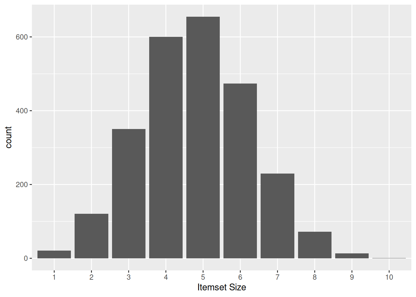
5.5 Association Rule Visualization*
Visualization is a very powerful approach to analyse large sets of mined association rules and frequent itemsets. We present here some options to create static visualizations and inspect rule sets interactively.
5.5.1 Static Visualizations
Default scatterplot
plot(rules)
## To reduce overplotting, jitter is added! Use jitter = 0 to prevent jitter.
Note that some jitter (randomly move points) was added to show how many rules have the same confidence and support value. Without jitter:
plot(rules, shading = "order")
## To reduce overplotting, jitter is added! Use jitter = 0 to prevent jitter.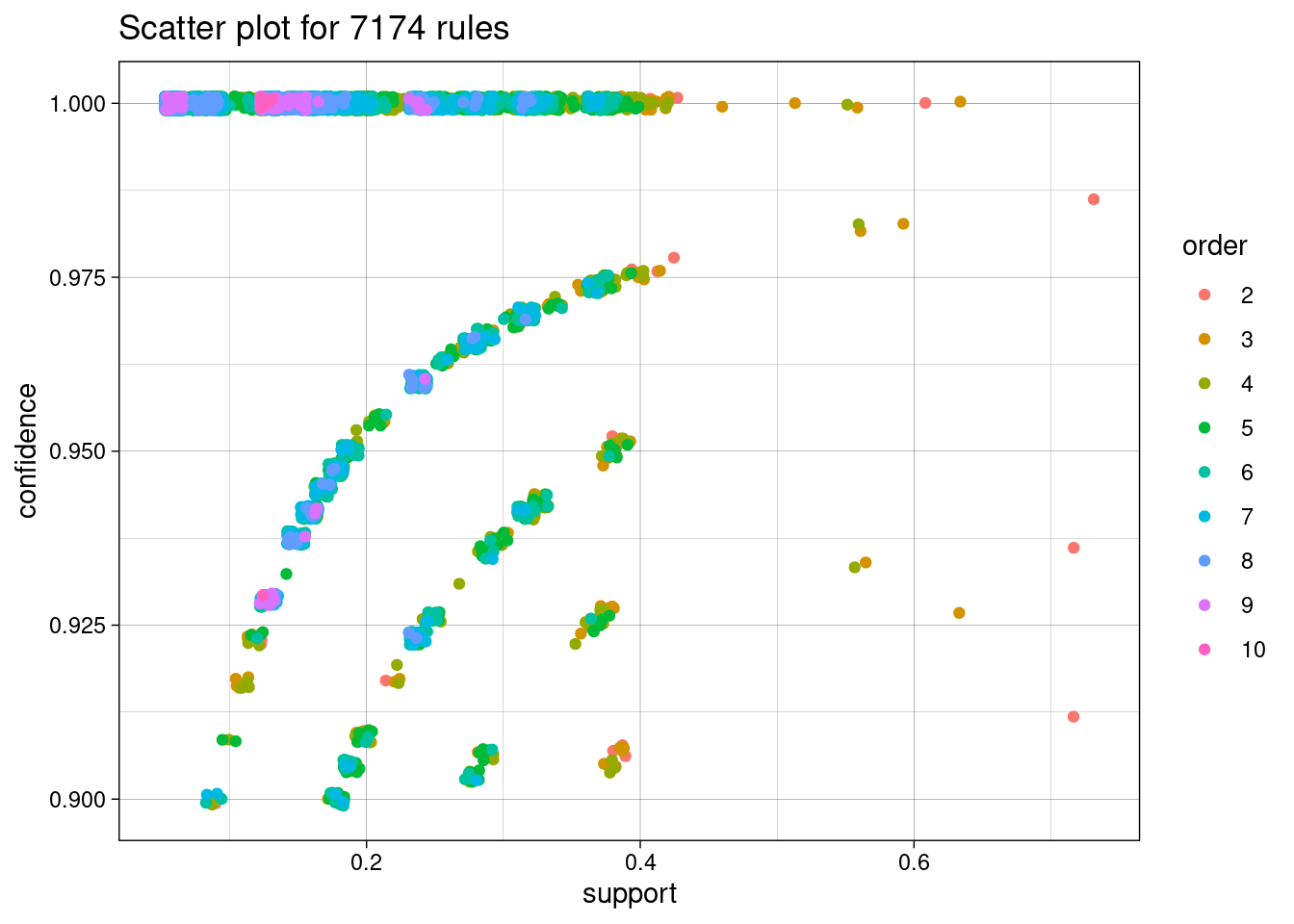
##plot(rules, interactive = TRUE)Grouped plot
plot(rules, method = "grouped")
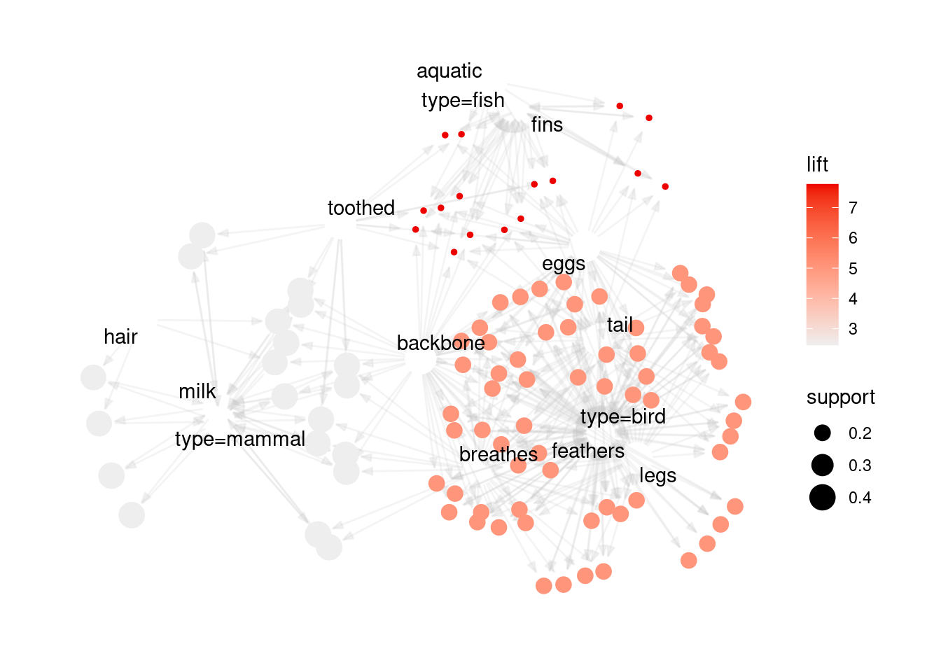
##plot(rules, method = "grouped", engine = "interactive")As a graph
plot(rules, method = "graph")
## Warning: Too many rules supplied. Only plotting the best 100 using
## 'lift' (change control parameter max if needed).
5.5.2 Interactive Visualizations
We will use the association rules mined from the Iris dataset for the following examples.
data(iris)
summary(iris)
##   Sepal.Length   Sepal.Width    Petal.Length   Petal.Width
##  Min.   :4.30   Min.   :2.00   Min.   :1.00   Min.   :0.1
##  1st Qu.:5.10   1st Qu.:2.80   1st Qu.:1.60   1st Qu.:0.3
##  Median :5.80   Median :3.00   Median :4.35   Median :1.3
##  Mean   :5.84   Mean   :3.06   Mean   :3.76   Mean   :1.2
##  3rd Qu.:6.40   3rd Qu.:3.30   3rd Qu.:5.10   3rd Qu.:1.8
##  Max.   :7.90   Max.   :4.40   Max.   :6.90   Max.   :2.5
##        Species
##  setosa    :50
##  versicolor:50
##  virginica :50
##
##
##
Convert the data to transactions.
iris_trans <- transactions(iris)
## Warning: Column(s) 1, 2, 3, 4 not logical or factor. Applying default
## discretization (see '? discretizeDF').
Note that this conversion gives a warning to indicate that some potentially unwanted conversion happens. Some features are numeric and need to be discretized. The conversion automatically applies frequency-based discretization with 3 classes to each numeric feature, however, the use may want to use a different discretization strategy.
iris_trans |> head() |> inspect()
##     items                      transactionID
## [1] {Sepal.Length=[4.3,5.4),
##      Sepal.Width=[3.2,4.4],
##      Petal.Length=[1,2.63),
##      Petal.Width=[0.1,0.867),
##      Species=setosa}                       1
## [2] {Sepal.Length=[4.3,5.4),
##      Sepal.Width=[2.9,3.2),
##      Petal.Length=[1,2.63),
##      Petal.Width=[0.1,0.867),
##      Species=setosa}                       2
## [3] {Sepal.Length=[4.3,5.4),
##      Sepal.Width=[3.2,4.4],
##      Petal.Length=[1,2.63),
##      Petal.Width=[0.1,0.867),
##      Species=setosa}                       3
## [4] {Sepal.Length=[4.3,5.4),
##      Sepal.Width=[2.9,3.2),
##      Petal.Length=[1,2.63),
##      Petal.Width=[0.1,0.867),
##      Species=setosa}                       4
## [5] {Sepal.Length=[4.3,5.4),
##      Sepal.Width=[3.2,4.4],
##      Petal.Length=[1,2.63),
##      Petal.Width=[0.1,0.867),
##      Species=setosa}                       5
## [6] {Sepal.Length=[5.4,6.3),
##      Sepal.Width=[3.2,4.4],
##      Petal.Length=[1,2.63),
##      Petal.Width=[0.1,0.867),
##      Species=setosa}                       6
Next, we mine association rules.
rules <- apriori(iris_trans, parameter = list(support = 0.1, confidence = 0.8))
## Apriori
##
## Parameter specification:
##  confidence minval smax arem  aval originalSupport maxtime support
##         0.8    0.1    1 none FALSE            TRUE       5     0.1
##  minlen maxlen target  ext
##       1     10  rules TRUE
##
## Algorithmic control:
##  filter tree heap memopt load sort verbose
##     0.1 TRUE TRUE  FALSE TRUE    2    TRUE
##
## Absolute minimum support count: 15
##
## set item appearances ...[0 item(s)] done [0.00s].
## set transactions ...[15 item(s), 150 transaction(s)] done [0.00s].
## sorting and recoding items ... [15 item(s)] done [0.00s].
## creating transaction tree ... done [0.00s].
## checking subsets of size 1 2 3 4 5 done [0.00s].
## writing ... [144 rule(s)] done [0.00s].
## creating S4 object  ... done [0.00s].
rules
## set of 144 rules5.5.2.2 Scatter Plot
Plot rules as a scatter plot using an interactive html widget. To avoid
overplotting, jitter is added automatically. Set jitter = 0 to disable
jitter. Hovering over rules shows rule information. Note:
plotly/javascript does not do well with too many points, so plot selects
the top 1000 rules with a warning if more rules are supplied.
plot(rules, engine = "html")
## To reduce overplotting, jitter is added! Use jitter = 0 to prevent jitter.
5.5.2.3 Matrix Visualization
Plot rules as a matrix using an interactive html widget.
plot(rules, method = "matrix", engine = "html") 5.5.2.4 Visualization as Graph
Plot rules as a graph using an interactive html widget. Note: the used javascript library does not do well with too many graph nodes, so plot selects the top 100 rules only (with a warning).
plot(rules, method = "graph", engine = "html")
## Warning: Too many rules supplied. Only plotting the best 100 using
## 'lift' (change control parameter max if needed).
5.5.2.5 Interactive Rule Explorer
You can specify a rule set or a dataset. To explore rules that can be
mined from iris, use: ruleExplorer(iris)
The rule explorer creates an interactive Shiny application that can be used locally or deployed on a server for sharing. A deployed version of the ruleExplorer is available here (using shinyapps.io).
5.6 Exercises*
We will again use the Palmer penguin data for the exercises.
library(palmerpenguins)
head(penguins)
## # A tibble: 6 × 8
##   species island    bill_length_mm bill_depth_mm flipper_length_mm
##   <chr>   <chr>              <dbl>         <dbl>             <dbl>
## 1 Adelie  Torgersen           39.1          18.7               181
## 2 Adelie  Torgersen           39.5          17.4               186
## 3 Adelie  Torgersen           40.3          18                 195
## 4 Adelie  Torgersen           NA            NA                  NA
## 5 Adelie  Torgersen           36.7          19.3               193
## 6 Adelie  Torgersen           39.3          20.6               190
## # ℹ 3 more variables: body_mass_g <dbl>, sex <chr>, year <dbl>- Translate the penguin data into transaction data with:
trans <- transactions(penguins)
## Warning: Column(s) 1, 2, 3, 4, 5, 6, 7, 8 not logical or factor.
## Applying default discretization (see '? discretizeDF').
## Warning in discretize(x = c(2007, 2007, 2007, 2007, 2007, 2007, 2007, 2007, : The calculated breaks are: 2007, 2008, 2009, 2009
##   Only unique breaks are used reducing the number of intervals. Look at ? discretize for details.
trans
## transactions in sparse format with
##  344 transactions (rows) and
##  22 items (columns)
Why does the conversion report warnings?
- What do the following first three transactions mean?
inspect(trans[1:3])
##     items                             transactionID
## [1] {species=Adelie,
##      island=Torgersen,
##      bill_length_mm=[32.1,40.8),
##      bill_depth_mm=[18.3,21.5],
##      flipper_length_mm=[172,192),
##      body_mass_g=[3.7e+03,4.55e+03),
##      sex=male,
##      year=[2007,2008)}                            1
## [2] {species=Adelie,
##      island=Torgersen,
##      bill_length_mm=[32.1,40.8),
##      bill_depth_mm=[16.2,18.3),
##      flipper_length_mm=[172,192),
##      body_mass_g=[3.7e+03,4.55e+03),
##      sex=female,
##      year=[2007,2008)}                            2
## [3] {species=Adelie,
##      island=Torgersen,
##      bill_length_mm=[32.1,40.8),
##      bill_depth_mm=[16.2,18.3),
##      flipper_length_mm=[192,209),
##      body_mass_g=[2.7e+03,3.7e+03),
##      sex=female,
##      year=[2007,2008)}                            3
Next, use the ruleExplorer() function to analyze association rules
created for the transaction data set.
Use the default settings for the parameters. Using the Data Table, what is the association rule with the highest lift. What does its LHS, RHS, support, confidence and lift mean?
Use the Graph visualization. Use select by id to highlight different species and different islands and then hover over some of the rules. What do you see?